Version History
There have been four major spm1d releases: 0.4, 0.3, 0.2 and 0.1.
The current major version is 0.4.
Release notes for previous versions are available here:
New Features
Version 0.4.8 (2021-09-09)
Equal variance test
eqvartest: a test for the equality of variance in two samples. This is a preliminary, in-development test based on the MATLAB code from Kowalski et al. (2021). Two alternative options are implemented: “unequal” or “greater”. The “unequal” alternative currently can be applied only if the sample sizes are equal. The “greater” alternative can be used for arbitrary sample sizes.
Here are links to an example Python script and an example MATLAB script.
Check the Python function or MATLAB function for additional details.
Version 0.4.3
Manual nonlinear warping (Python only)
Nonlinearly warp 1D data to improve alignment of homologous events.
Warp data using “landmark” and “manual” modes.
Full documentation: mwarp1d
Version 0.4.2
Analysis of 2D data using spm1d:
Version 0.4.0
The main new features in spm1d version 0.4 are listed below.
Note
Additional documentation will be added following peer review.
Non-parametric inference
All statistical tests can now be conducted non-parametrically through the new spm1d.stats.nonparam interface.
Example (0D parametric):
>>> import spm1d
>>> yA = [1, 2, 4, 1, 2, 3, 2, 2]
>>> yB = [3, 2, 3, 4, 2, 5, 4, 3]
>>> t = spm1d.stats.ttest2(yA, yB)
>>> ti = t.inference(0.05)
>>> print(ti)
Example (0D non-parametric):
>>> tn = spm1d.stats.nonparam.ttest2(yA, yB)
>>> tni = tn.inference(0.05, iterations=1000)
>>> print(tni)
The key difference is the “iterations” keyword for non-parametric inference. This sets the number of random data permutations used. Setting iterations to “-1” performs all possible permutations.
Note
spm1d’s non-parametric procedures follow Nichols & Holmes (2002). Please consider citing:
Nichols TE, Holmes AP (2002). Nonparametric permutation tests for functional neuroimaging: a primer with examples. Human Brain Mapping 15(1), 1–25.
Confidence intervals
Parametric and non-parametric confidence intervals (CIs) can be constructed using the following functions:
Parametric:
spm1d.stats.ci_onesample
spm1d.stats.ci_pairedsample
spm1d.stats.ci_twosample
Non-parametric:
spm1d.stats.nonparam.ci_onesample
spm1d.stats.nonparam.ci_pairedsample
spm1d.stats.nonparam.ci_twosample
For more details refer the example scripts listed below. The standalone scripts construct CIs outside of spm1d and show all computational details.
./spm1d/examples/stats0d/
ex_ci_onesample_standalone.py
ex_ci_onesample.py
ex_ci_pairedsample.py
ex_ci_twosample.py
./spm1d/examples/stats1d/
ex_ci_onesample_standalone.py
ex_ci_onesample.py
ex_ci_pairedsample.py
ex_ci_twosample.py
./spm1d/examples/nonparam/0d/
ex_ci_onesample.py
ex_ci_pairedsample.py
ex_ci_twosample.py
./spm1d/examples/nonparam/1d/
ex_ci_onesample.py
ex_ci_pairedsample.py
ex_ci_twosample.py
Normality tests
Normality tests can be conducted using the new spm1d.stats.normality interface.
The normality assessments currently available include:
D’Agostino-Pearson K2 test (spm1d.stats.normality.k2)
Shapiro-Wilk statistic (spm1d.stats.normality.sw)
spm1d provides convenience functions for all statistical procedures, making it easy to assess normality for arbitrary designs.
For example:
>>> t  = spm1d.stats.regress(y, x)                #linear regression test statistic (t value)
>>> ti = t.inference(0.05)                        #assess whether the observed linear correlation is significant
>>> n  = spm1d.stats.normality.k2.regress(y, x)   #normality test statistic (K2)
>>> ni = spm.inference(0.05)                      #assesses whether the observed non-normality is significant
Python 3 compatibility
FINALLY!
spm1d is now compatible with both Python 2.7 and Python 3.5
Python 2.7 and Python 3.X will both be supported for the forseeable future.
Note
As of May 2021, Python 2.X is no longer supported. Please use Python 3.8 or newer.
rft1d in spm1d
The rft1d package, which spm1d uses to compute probabilities, is now packaged inside spm1d.
All rft1d updates will be pushed to spm1d, so now you only need to keep spm1d up-to-date.
Improved ANOVA interface
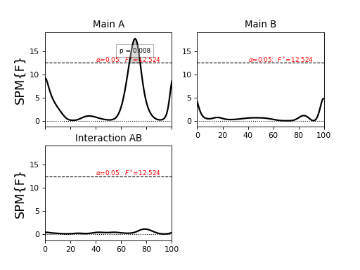
Results from two- and three-way ANOVA are now much easier to summarize, visualize and navigate.
Example (two-way ANOVA for 1D data):
>>> dataset      = spm1d.data.uv1d.anova2.SPM1D_ANOVA2_2x2()
>>> Y,A,B        = dataset.get_data()
Here Y is the data array, and A and B are vectors containing experimental condition labels as integers, one integer label for each row of Y.
>>> FF           = spm1d.stats.anova2(Y, A, B, equal_var=True)
>>> FFi          = FF.inference(0.05)
>>> print( FFi )
The “print” statement prints the following ANOVA summary to the screen:
SPM{F} inference list
   design    :  ANOVA2
   nEffects  :  3
Effects:
   A     z=(1x101) array      df=(1, 16)   h0reject=True
   B     z=(1x101) array      df=(1, 16)   h0reject=False
   AB    z=(1x101) array      df=(1, 16)   h0reject=False
The main effects A and B and the interaction effect AB are listed along with the degrees of freedom and the null hypothesis rejection decision.
The specific effects can be accessed using either integers:
>>>  FAi  = FFi[0]   #main effect of A
>>>  FBi  = FFi[1]   #main effect of B
>>>  FABi = FFi[2]   #interaction effect
or the new more intuitive interface:
>>>  FAi  = FFi['A']
>>>  FBi  = FFi['B']
>>>  FABi = FFi['AB']
Each effect itself contains detailed information:
>>> print( FAi )
SPM{F} inference field
   SPM.effect    :   Main A                        #effect name
   SPM.z         :  (1x101) raw test stat field    #test statistic field
   SPM.df        :  (1, 16)                        #degrees of freedom
   SPM.fwhm      :  14.28048                       #field smoothness
   SPM.resels    :  (1, 7.00257)                   #resolution element counts
Inference:
   SPM.alpha     :  0.050                          #user-selected Type I error rate
   SPM.zstar     :  12.52450                       #critical test statistic value
   SPM.h0reject  :  True                           #null hypothesis rejection decision
   SPM.p_set     :  0.008                          #set-level probability
   SPM.p_cluster :  (0.008)                        #cluster-level probabilities
Last, the results can plotted much more easily than before, now with a single command:
>>>  pyplot.close('all')
>>>  FFi.plot(plot_threshold_label=True, plot_p_values=True, autoset_ylim=True)
>>>  pyplot.show()
(Source code, png, hires.png, pdf)

Version 0.3.2
Region-of-Interest (ROI) analysis.
All statistical routines in spm1d.stats now accept a keyword “roi” for conducting ROI analysis.
Note
Update! (2016.11.02) ROI analysis details are available in:
Pataky TC, Vanrenterghem J, Robinson MA (2016). Region-of-interest analyses of one-dimensional biomechanical trajectories: bridging 0D and 1D methods, augmenting statistical power. PeerJ 4: e2652, doi.org/10.7717/peerj.2652.
See the Appendix for a description of spm1d’s interface for ROI analysis.
Version 0.3.1
This update contains major edits to the ANOVA code.
Newly supported ANOVA models:
spm1d.stats.anova3rm (three-way design with repeated-measures on all three factors)
spm1d.stats.anova2onerm (now supports unbalanced designs: i.e. different numbers of subjects for each level of factor A)
WARNING: Repeated-measures ANOVA
IF (a) the data are 1D and (b) there is only one observation per subject and per condition…
THEN inference is approximate, based on approximated residuals.
TO AVOID THIS PROBLEM: use multiple observations per subject per condition, and the same number of observations across all subjects and conditions.
WARNING: Non-sphericity corrections
Now only available for two-sample t tests and one-way ANOVA.
The correction for one-way ANOVA is approximate and has not been validated.
Non-sphericity corrections for other designs are currently being checked.
Version 0.3
The main new features in spm1d version 0.3 are:
M-way repeated measures ANOVA
spm1d now supports a variety of M-way repeated measures and nested ANOVA designs:
- One-way
spm1d.stats.anova1 — one-way ANOVA
spm1d.stats.anova1rm — one-way repeated-measures ANOVA
- Two-way
spm1d.stats.anova2 — two-way ANOVA
spm1d.stats.anova2nested — two-way nested ANOVA
spm1d.stats.anova2rm — two-way repeated-measures ANOVA
spm1d.stats.anova2onerm — two-way ANOVA with repeated measures on one factor
- Three-way
spm1d.stats.anova3 — three-way ANOVA
spm1d.stats.anova3nested — three-way fully nested ANOVA
spm1d.stats.anova3onerm — three-way ANOVA with repeated measures on one factor
spm1d.stats.anova3tworm — three-way ANOVA with repeated measures on two factors
Warning
Currently unsupported ANOVA functionality includes:
Non-sphericity corrections for two- and three-way repeated-measures designs
Unbalanced designs for M > 1
Missing data
Mixed (fixed and random factor) designs. Mixed effects analysis should be implemented using the hierarchical procedure described here
Abitrary designs (Latin Square, partially nested, etc.)
Multivariate analysis
spm1d now supports basic analyses of multivariate 1D continua:
spm1d.stats.hotellings — one-sample Hotelling’s T2 test
spm1d.stats.hotellings_paired — paired Hotelling’s T2 test
spm1d.stats.hotellings2 — two-sample Hotelling’s T2 test
spm1d.stats.cca — canonical correlation analysis (univariate 0D independent variable and multivariate 1D dependent variable)
spm1d.stats.manova1 — one-way multivariate analysis of variance.
Warning
Non-sphericity corrections are not yet implemented for relevant multivariate procedures including:
Hotelling’s two-sample T2
MANOVA
0D analysis
All spm1d.stats functions now support both 0D and 1D data data analysis.
Example (0D):
>>> yA = [1, 2, 2, 1, 3]
>>> yB = [3, 1, 2, 3, 4]
>>> t = spm1d.stats.ttest2(yA, yB)
>>> ti = t.inference(0.05)
>>> print( ti )  #display inference results
Example (1D):
>>> yA = np.random.randn(5,101)
>>> yB = np.random.randn(5,101)
>>> t = spm1d.stats.ttest2(yA, yB)
>>> ti = t.inference(0.05)
>>> ti.plot()  #plot inference results
Find more details in the example scripts in ./spm1d/examples/stats0d/
The scripts compare spm1d results to third-party results (from SAS, SPSS, Excel, R, etc.) for a variety of datasets available on the web.
MATLAB syntax == Python syntax
spm1d’s MATLAB and Python syntaxes are now nearly identical.
Example two-sample t test (Python):
>>> yA = np.random.randn(8,101)
>>> yB = np.random.randn(8,101)
>>> t  = spm1d.stats.ttest2(yA, yB)
>>> ti = t.inference(0.05)
Example two-sample t test (MATLAB):
>>> yA = randn(8,101);
>>> yB = randn(8,101);
>>> t  = spm1d.stats.ttest2(yA, yB);
>>> ti = t.inference(0.05);
Datasets
A variety of 0D and 1D datasets are now available:
spm1d.data.uv0d — univariate 0D datasets
spm1d.data.uv1d — univariate 1D datasets
spm1d.data.mv0d — multivariate 0D datasets
spm1d.data.mv1d — multivariate 1D datasets
Inference
spm1d now uses the rft1d package for conducting statistical inference.
The following features are supported:
Set-level inference (previously only cluster-level inference was available)
Circular fields (i.e. 0% and 100% are homologous, like the calendar year or the gait stride cycle)
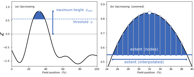
Cluster interpolation (to the critical threshold for more accurate p values)
Warning
Other rft1d procedures like broken-field analysis and element- vs. node-based inferences will be integrated in future versions of spm1d.
Set-level inference
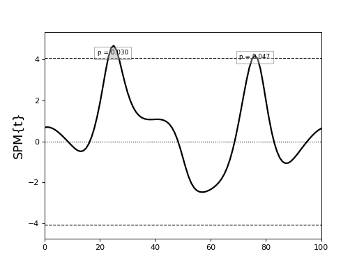
Consider the following example:
import spm1d
YA,YB = spm1d.data.uv1d.t2.SimulatedTwoLocalMax().get_data()
t = spm1d.stats.ttest2(YB, YA)
ti = t.inference(0.05)
ti.plot()
ti.plot_p_values()
(Source code, png, hires.png, pdf)

This yields the following results:
SPM{T} inference field
        SPM.z         :  (1x101) raw test stat field
        SPM.df        :  (1, 9.894)
        SPM.fwhm      :  13.63026
        SPM.resels    :  (1, 7.33662)
Inference:
        SPM.alpha     :  0.050
        SPM.zstar     :  4.07916
        SPM.h0reject  :  True
        SPM.p_set     :  <0.001
        SPM.p_cluster :  (0.015, 0.023)
The cluster-level p values are 0.015 and 0.023, but the set-level p value (<0.001) is much lower.
Note
Interpreting probabilities
Cluster-level p value : the probability that 1D Gaussian random fields with the observed smoothness would produce a suprathreshold cluster with an extent as large as the observed cluster’s extent.
Set-level p value : the probability that 1D Gaussian random fields with the observed smoothness would produce C suprathreshold clusters, all with extents larger than the minimum observed extent.
Set- and cluster-level probabilities are identical when there is just one suprathreshold cluster.
Circular fields
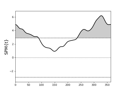
If the first point in the 1D field is homologous with the last point, like in calendar years or gait strides, then the field is ‘circular’.
Consider the following example from Ramsay JO, Silverman BW (2005). Functional Data Analysis (Second Edition), Springer, New York.
Click here for a description of this dataset
import spm1d
dataset  = spm1d.data.uv1d.anova1.Weather()
Y,A      = dataset.get_data()
Y0,Y1    = Y[A==0], Y[A==2]  #Atlantic and Contintental regions
t        = spm1d.stats.ttest2(Y0, Y1)
ti       = t.inference(0.05, circular=True)
ti.plot()
(Source code, png, hires.png, pdf)

There appear to be two suprathreshold clusters, but Day 0 is homologous with Day 365, so in fact there is just one suprathreshold cluster.
If the example above is regarded as circular, we get a single cluster-level p value of approximately 0.000003.
If instead it is regarded as non-circular, we get two cluster-level p values of approximately 0.006 and 0.001.
Note
Use the keyword circular when conducting inference to specify whether or not the field is circular.
>>> ti = t.inference(0.05, circular=True)
By default circular is False.
Cluster interpolation
spm1d now interpolates to the critical threshold u as depicted in panel (b) of the figure below.
Interpolation is conducted by deault, but can be toggled using the interp keyword for inference:
>>>  t = spm1d.stats.ttest(YA, YB)
>>>  ti = t.inference(0.05, interp=True)
>>>  ti = t.inference(0.05, interp=False)
(Source code, png, hires.png, pdf)

Installation & Updating
The Python version of spm1d can be now installed and updated from the command line:
easy_install spm1d
Source code for both Python and MATLAB can be cloned and updated from github.com.
