Overview of random effects analysis¶

If one’s hypothesis pertains to a population of subjects, or multiple populations of subjects, then spm1d can be used to conduct random effects analysis (RFX) using a hierarchical (two-level) random effects model:

Level 1 — estimate within-subject effect(s) (” β “) using one experimental model (e.g. regression, t test, etc.) for each subject.
Level 2 — test estimated effects (” β “) using a separate population-level model.

The RFX approach is described in detail in References [4] and [6]

Hypothetical experiment¶

Consider a simple experiment:

Subjects — Group A (8 subjects), Group B (8 subjects)
Task — One experimental task (“Task T”)
Repetitions — Five per subject (TOTAL = 80 measurements)
Dependent variable — One scalar y
Null hypothesis — No difference in the Group A mean y and the Group B mean y when performing Task T.

Hierarchical RFX analyses would proceed as follows:

Level 1: compute the mean y value for each subject (i.e. compute β for each subject).
Level 2: conduct a two-sample or paired t test on the resulting β parameters.

Explanation:

This hierarchical RFX approach regards each β as a random variable. In other words, each subect’s β is considered to have been sampled randomly from a larger population.
This approach is especially useful when within-subject variability is small relative to between-subject variability. Consider a case where within-subject variability is ten times smaller than between-subject variability. In such an experiment, we could measure each subject just once (instead of five times) without greatly affecting the results.
Repeated measurements on each subject leads to more accurate measurements of each subject’s β, implying that between-subject differences generally become more stable as one performs more measurements on each subject.

We shall see that these basic RFX concepts apply equivalently to 1D continuum analysis.

Example analysis¶

./spm1d/examples/stats1d/rfx_0_means.py

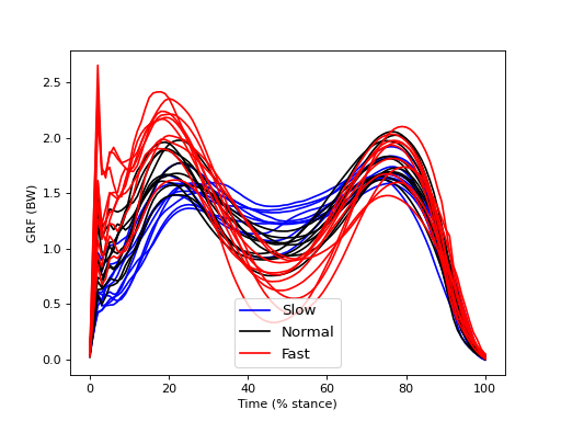
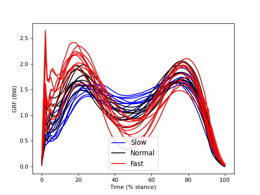
This dataset examines the effects of walking speed on vertical ground reaction forces (GRF) in ten subjects. Each performed 20 trials of each of Slow, Normal, and Fast walking and all GRF trajectories were normalized in time by stance phase (% stance) and in magnitude by body weight (BW). Since we are interested in whether measured SPEED-GRF effects extrapolate to the broader population of subjects from which these ten were drawn, our null hypothesis is: no between-subject effect of SPEED on GRF. In other words, we are not interested in an a priori sense whether or not particular subjects exhibit SPEED-GRF effects. We are only interested in whether SPEED-GRF effects are systematic across subjects.

The figure below depicts within-subject mean GRF continua for each of the three SPEED conditions. Despite rather large between-subject variability there appear to be various systematic effects of walking speed on the GRF trajectory. For example, there appears to be a postive correlation between SPED and GRF in early stance (before 20%).

Note

The between-subject variability depicted in the figure below is relatively large compared the to within-subject variability depicted in the main regression example.

(Source code, png, hires.png, pdf)

Level 1 Analysis¶

./spm1d/examples/stats1d/rfx_1_level1.py

To model the effect of SPEED on GRF within each subject, we can use a linear regression model, just like in the the main regression example:

Note

Although the figure above depicts the data categorically (in three different speed categories), the independent variable (SPEED) is actually a continuous variable, which was measured experimentally. Thus regression is a more appropriate within-subject model than is one-way ANOVA.

>>>  subj = 0
>>>  Y,x  = spm1d.util.get_dataset('speed-grf', subj)
>>>  t    = spm1d.stats.regress(Y, x)

Danger

Our null hypothesis does not pertain to within-subject effects. We therefore mustn’t conduct inference on within-subject effects, like we did elsewhere in a single-subject experiment.

Warning

Do not misinterpret β parameter computation as equivalent to statistical testing. Similar to basic test statistic continuum computation, statistical “testing” only occurs when one conducts statistical inference — i.e. critical threshold and/or probability value computation.

After conducting within-subject regression, each subject’s regression parameters β may be extracted using the SPM object’s beta attribute:

>>>  t    = spm1d.stats.regress(Y, x)
>>>  beta = t.beta

Note the shape of the β parameter array:

>>>  print( beta.shape )

(2, 101)

There are two β parameter continua, each sampled at 101 nodes (like the original data). The two β parameters correspond to the linear regression slope and intercept, respectively. We may retrieve the first β parameter using simple array indexing:

Warning

Our hypothesis pertains only to regression slope (the first β parameter), which embodies the effect of SPEED on GRF.

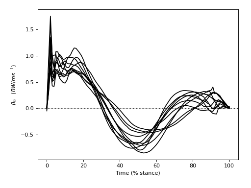
>>>  beta0 = t.beta[0]

The figure below depicts all β continua — one for each of the ten subjects. Positive and negative β imply positive and negative correlation, respectively, between SPEED and GRF. We can see that all subjects appear to have exhibited similar β continua, and that the mean β continuum is qualitatively different from the null continuum (which is depicted as a dotted line).

Note

If our null hypothesis were true, and there were truly no effect of SPEED on GRF, we would expect each subject’s β continuum to be quite different. In particular, we would expect the mean between-subject β continuum to converge to the null continuum as the number of subjects increases. The goal of Level 2 analysis is to quantify the likelihood that smooth, random continua would yield a set of β continua that similarly diverge from the null continuum.

(Source code, png, hires.png, pdf)

To appreciate the meaning of the β parameters, consider the simple regression model:

$y = \beta_0 x + \beta_1 + \varepsilon$

The first and second β parameters are clearly the slope and intercept. In spm1d arbitrary models like this are fit to the data at each continuum node, to generate one-dimensional β parameter continua.

Level 2 Analysis¶

./spm1d/examples/stats1d/rfx_2_level2.py

If our null hypothesis were true we would expect no systematic difference between a group of β continua and the null continua. We can therefore submit the β continua to a one-sample t test, where the datum is the null continuum. First we assemble the BETA parameters for each subject as follows:

>>> nSubj    = 10
>>> BETA     = []  #regression slopes
>>> for subj in range(nSubj):
>>>     Y,x  = spm1d.util.get_dataset('speed-grf', subj)  #load data
>>>     t    = spm1d.stats.regress(Y, x) #conduct linear regression
>>>     BETA.append( t.beta[0] )  #retrieve the regression slope
>>> BETA     = np.array(BETA)

Now BETA is a (10 x 101) array contining our β continuum estimates, one continuum per subject. These β continua become the dependent variable for Level 2 analysis, as follows:

>>> alpha = 0.05
>>> t     = spm1d.stats.ttest(BETA)
>>> ti    = t.inference(alpha, two_tailed=True)
>>> ti.plot()

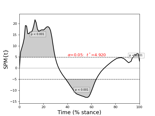
The figure below depcits the resulting SPM{t}, which exceeds the critical threshold at various points in the continuum. From a classical hypothesis testing perspective we can therefore reject the null hypothesis of no between-subject effect of SPEED on GRF at a Type I error rate of α.

A verbose interpretation of “p < 0.001” is: “Gaussian random fields of the identical smoothness as the observed residuals, and as long as the observed continua, would produce a suprathreshold cluster as large as the observed cluster in fewer than 0.1% of many repeated experiments.”

(Source code, png, hires.png, pdf)

Danger

These results do not prove that there is, in fact, a real effect of SPEED on GRF. The results mean one thing and one thing only: random data would produce similar results relatively infrequently. The null hypothesis is generally falsifiable only through repeated experimentation, and an accumulation of scientific evidence. This notion is formally embodied in Bayesian inference, but is currently not implemented in spm1d.

Warning

Had we chosen a different model, for example: two-way ANOVA with SUBJECT and SPEED as factors, both SUBJECT and SPEED would have been fixed. This is quite different to the Level 2 analysis above, which regards SUBJECT as random. If SUBJECT is fixed, inference pertains only to those subjects, and not to the larger population from which those subjects were drawn. Conversely, modeling SUBJECT as random allows us to extrapolate to the larger population.