Power analysis

One-sample

Here the Canadian temperature dataset from the previous section will be used to demonstrate one-sample power analysis.

A full script for one-sample power analysis appears below, and immediately below that we shall consider it in more detail.

import power1d

J        = 8    # sample size
Q        = 365  # continuum size

# construct baseline geometry:
g0       = power1d.geom.GaussianPulse( Q , q=200 , fwhm=190 , amp=40 )
g1       = power1d.geom.Constant( Q , amp=23 )
baseline = g0 - g1  # subtract the geometries

# construct signal geometry:
signal0  = power1d.geom.Null( Q )
signal1  = power1d.geom.GaussianPulse( Q , q=200 , fwhm=100 , amp=5 )

# construct noise model:
noise0   = power1d.noise.Gaussian( J , Q , mu = 0 , sigma = 0.3 )
noise1   = power1d.noise.SmoothGaussian( J , Q , mu = 0 , sigma = 3 , fwhm = 70 )
noise    = power1d.noise.Additive( noise0 , noise1 )

# create data sample models:
model0   = power1d.models.DataSample( baseline, signal0, noise, J=J )
model1   = power1d.models.DataSample( baseline, signal1, noise, J=J )

# create experiment models:
teststat = power1d.stats.t_1sample
emodel0  = power1d.models.Experiment( model0 , teststat )    # null hypothesis
emodel1  = power1d.models.Experiment( model1 , teststat )    # alternative hypothesis

# simulate the experiments:
sim      = power1d.ExperimentSimulator( emodel0 , emodel1 )
results  = sim.simulate( 5000, progress_bar=True )

# visualize the power results:
results.plot()

(Source code, png, hires.png, pdf)

All of the commands from the code above up until “# create experiment models” are describe in the previous section regarding data modeling. The only difference is that here two signals and two data sample models are created: one representing the null hypothesis and one representing the alternative hypothesis. In power1d the “Null” geometry is a null continuum (i.e. a continuum with all zero values) as seen here.

Once the signals and data samples are constructed, the next step is to add them to a power1d.models.Experiment object along with a test statistic function. When there is just one data sample model the test statistic function should accept a (J x Q) data array and return a (Q,) array representing the test statistic continuum. Test statistic functions for a variety of common experimental designs are available in power1d.stats.

Next the two Experiment models, representing the null and alternative hypotheses are added to an ExperimentSimulator object. When the simulate method is called for N iterations (here N$=5000) the simulator will simualte both the null and the alternative experiments for *N iterations and store the test statistic continua for both as (N x Q) arrays in the results.Z0 and results.Z1 attributes, respectively.

Last, the simulation results are summarized graphically using the plot method.

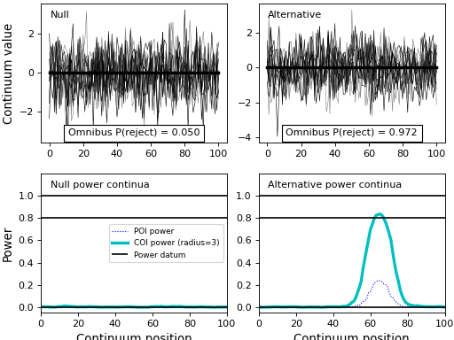
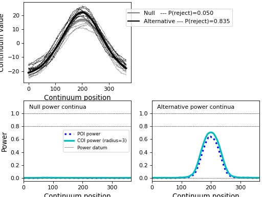
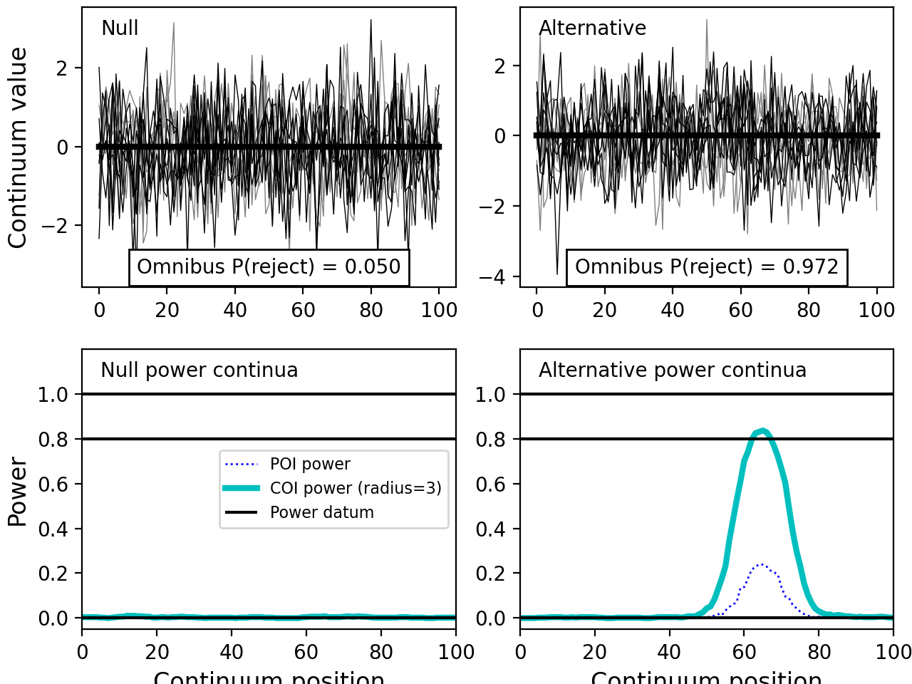
The top left panel of the results depicts the null and alternative models and lists their omnibus powers. By definition the ‘power’ of the null model is alpha, and alpha is 0.05 by default. Alpha and all other power-relevant parameters can be changed using the the results.set_ methods as summarized in the power1d.results API.

Here the alternative model has an omnibus power of 0.843. This sugges that, if our noise models are correct, we will reject the null hypothesis (of null signal) with a probability of 0.843. However, this doesn’t imply that we will detect the modeled signal with a probability of 0.843 because occassionally we will detect ‘signal’ which randomly appears in continuum regions outside of the signal region. This point is emphasized in the point-of-interest (POI) and center-of-interest (COI) power continua in the lower right panel. The POI continuum indicates the probability of rejecting the null hypothesis at particular continuum points, and the COI continuum indicates the same but extends the search region to a certain radius (here 3 points) around the POI. The POI and COI continuum results suggest that we are only about 70% likely to detect the signal we have modeled, even though the omnibus power is greater than 80%.

If we were to broaden the COI radius to the full continuum size of $Q$=365 using results.set_coi_radius(365), the COI continuum would plateau at the omnbus power of 0.843. Thus the POI and COI continua quantify the regional specificity of the omnibus power results.

Two-sample

A slightly simpler model than the one above will be used to demonstrate power calculations for two-sample and other experiments.

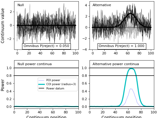
In the example below signal is modeled as a GaussianPulse at point 65 in a continuum of length 101 and noise is modeled as uncorreletated Gaussian. The two-sample test statistic function (power1d.stats.t_2sample_fn) is used to calculate the test statistic continuum

Note that power1d.stats functions with “_fn” appended to the end are slightly more efficient calculators than are those without “_fn” appended. This is because the “_fn” functions store calculations results like matrix inversion results so that they don’t have to be repeated across every single simulation iteration. More details regarding this are provided in power1d.stats.

Also note that, unlike the one-sample results above, power1d separates the null and alternative models into separate panels. This is done to prevent single-panel clutter.

import numpy as np
import power1d

#(0) Create geometry and noise models:
JA,JB,Q   = 5, 7, 101
baseline  = power1d.geom.Null(Q=Q)
signal0   = power1d.geom.Null(Q=Q)
signal1   = power1d.geom.GaussianPulse(Q=101, q=65, amp=2.5, sigma=10)
noise     = power1d.noise.Gaussian(J=5, Q=101, sigma=1)

#(1) Create data sample models:
modelA0   = power1d.models.DataSample(baseline, signal0, noise, J=JA) #null A
modelB0   = power1d.models.DataSample(baseline, signal0, noise, J=JB) #null N
modelA1   = power1d.models.DataSample(baseline, signal0, noise, J=JA) #alternative A
modelB1   = power1d.models.DataSample(baseline, signal1, noise, J=JB) #alternative B

#(2) Create experiment models:
teststat  = power1d.stats.t_2sample_fn(JA, JB)
expmodel0 = power1d.models.Experiment([modelA0, modelB0], teststat) #null
expmodel1 = power1d.models.Experiment([modelA1, modelB1], teststat) #alternative

#(3) Simulate experiments:
np.random.seed(0)
sim       = power1d.ExperimentSimulator(expmodel0, expmodel1)
results   = sim.simulate(1000, progress_bar=True)
results.plot()

(Source code, png, hires.png, pdf)

Regression

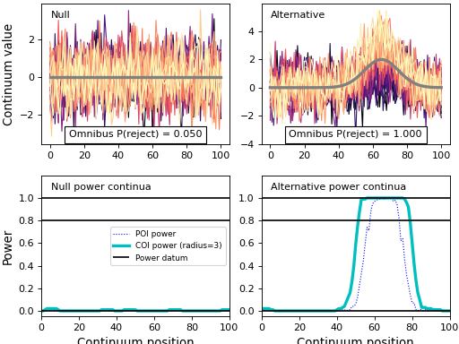
Regression can be implemented using the “regressor” keyword argument when constructing a DataSample model as indicated below.

Note that regression models are plotted with a different color scheme from those above: dark and bright colors correspond to small and large regressor values, respectively. In the “Alternative” model below (top right panel) it is apparent that dependent variable values get larger in the vicinity of Q=65 as the regressor values get larger, implying positive correlation between the independent and dependent variables in this vicinity.

import numpy as np
import power1d

#(0) Create geometry and noise models:
J,Q       = 30, 101
x         = np.linspace(0, 2, J)  #regressor (must have J values)
baseline  = power1d.geom.Null(Q=Q)
signal0   = power1d.geom.Null(Q=Q)
signal1   = power1d.geom.GaussianPulse(Q=101, q=65, amp=2.0, sigma=10)
noise     = power1d.noise.Gaussian(J=5, Q=101, sigma=1)

#(1) Create data sample models:
model0    = power1d.models.DataSample(baseline, signal0, noise, J=J, regressor=x)
model1    = power1d.models.DataSample(baseline, signal1, noise, J=J, regressor=x)

#(2) Create experiment models:
teststat  = power1d.stats.t_regress_fn(x)
expmodel0 = power1d.models.Experiment(model0, teststat)
expmodel1 = power1d.models.Experiment(model1, teststat)

#(3) Simulate experiments:
np.random.seed(0)
sim       = power1d.ExperimentSimulator(expmodel0, expmodel1)
results   = sim.simulate(100, progress_bar=True)
results.plot()

(Source code, png, hires.png, pdf)

One-way ANOVA

Power analyses for one-way ANOVA can be conducted almost identically to the two-sample analysis described above. The only difference is that more DataSample models are needed to represent each of the groups.

import numpy as np
import power1d

#(0) Create geometry and noise models:
JA,JB,JC,Q = 5, 7, 12, 101
baseline   = power1d.geom.Null(Q=Q)
signal0    = power1d.geom.Null(Q=Q)
signal1    = power1d.geom.GaussianPulse(Q=101, q=65, amp=1.5, sigma=10)
noise      = power1d.noise.Gaussian(J=5, Q=101, sigma=1)

#(1) Create data sample models:
modelA0   = power1d.models.DataSample(baseline, signal0, noise, J=JA)  #null A
modelB0   = power1d.models.DataSample(baseline, signal0, noise, J=JB)  #null B
modelC0   = power1d.models.DataSample(baseline, signal0, noise, J=JC)  #null C
modelA1   = power1d.models.DataSample(baseline, signal0, noise, J=JA)  #alternative A
modelB1   = power1d.models.DataSample(baseline, signal0, noise, J=JB)  #alternative B
modelC1   = power1d.models.DataSample(baseline, signal1, noise, J=JC)  #alternative C

#(2) Create experiment models:
teststat  = power1d.stats.f_anova1_fn(JA, JB, JC)
expmodel0 = power1d.models.Experiment([modelA0, modelB0, modelC0], teststat)
expmodel1 = power1d.models.Experiment([modelA1, modelB1, modelC1], teststat)

#(3) Simulate experiments:
np.random.seed(0)
sim       = power1d.ExperimentSimulator(expmodel0, expmodel1)
results   = sim.simulate(500, progress_bar=True)
results.plot()

(Source code, png, hires.png, pdf)