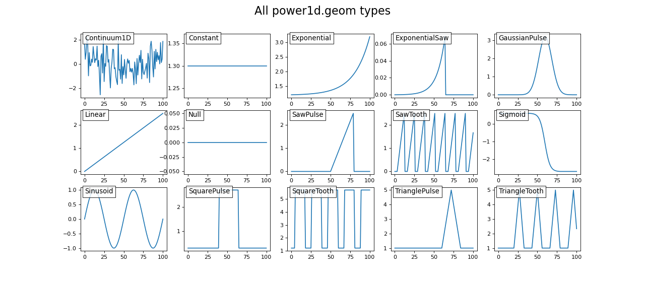
power1d.geom

One-dimensional (1D) continuum geometry primitives.

The classes in this module represent a set of building blocks for constructing 1D baselines and signals.

More complex 1D geometries can be constructed by combining multiple primitives through the standard operators: + - * / **

The figure below provides an overview of all geometric primitive types. Details regarding reach are listed below.

(Source code, png, hires.png, pdf)

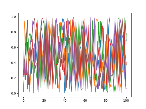
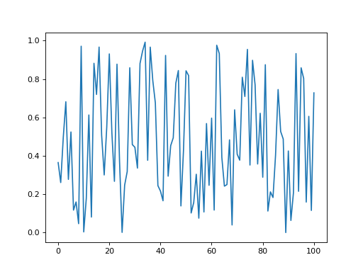
from_array

power1d.geom.from_array(x)

Create Continuum1D geometry object(s) from a 1D or 2D array.

Arguments:

x —- 1- or 2-dimensional numpy array

Outputs:

obj —- a Continuum1D object

Example:

import numpy as np
import power1d

x     = np.random.rand( 101 )
obj   = power1d.geom.from_array( x ) # Continuum1D object
obj.plot()

x     = np.random.rand( 5, 101 )
objs  = power1d.geom.from_array( x ) # list of Continuum1D objects
[obj.plot()  for obj in objs]

(Source code, png, hires.png, pdf)

from_file

power1d.geom.from_file(fpath)

Create Continuum1D geometry object(s) from a CSV file.

Only CSV files are currently supported.

1D arrays can be saved as either a single row or a single column in a CSV file.

2D arrays must be saved with shape (nrow,ncol) where nrow is the number of 1D arrays and each row will be converted to a Continuum1D object

Arguments:

fpath —- full path to a CSV file

Outputs:

obj —- a Continuum1D object

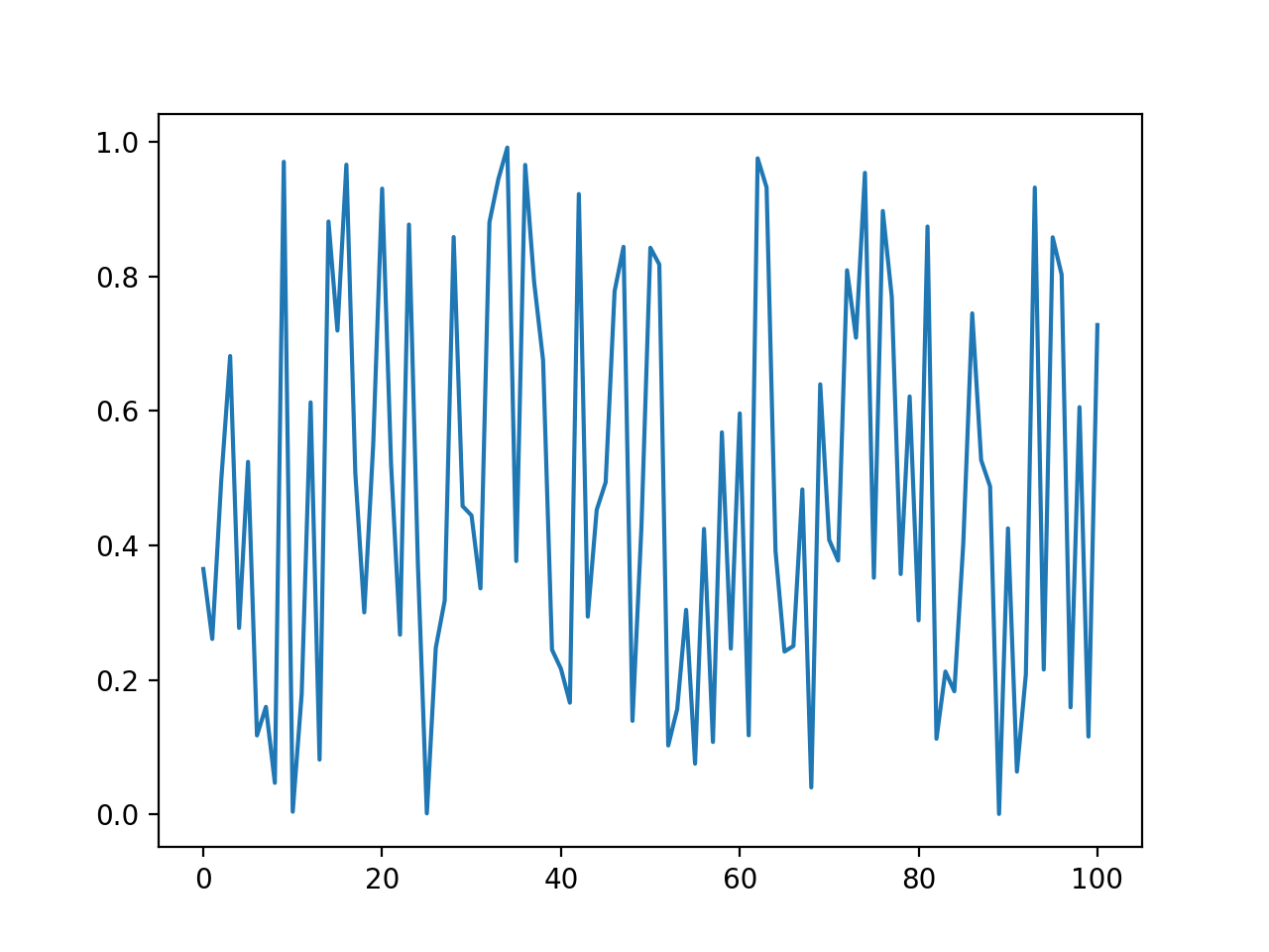
Continuum1D

power1d.geom.Continuum1D(value)

Manually defined one-dimensional continuum geometry.

Arguments:

value —- one-dimensional numpy array

Example:

import numpy as np
import power1d

value = np.random.rand( 101 )
obj   = power1d.geom.Continuum1D( value )
obj.plot()

(Source code, png, hires.png, pdf)

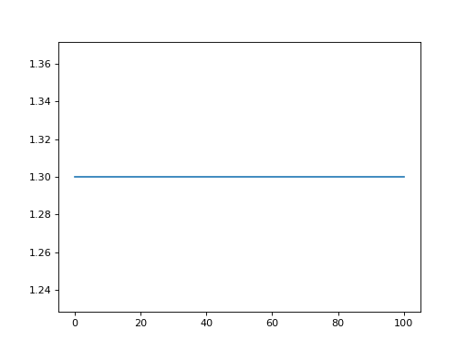
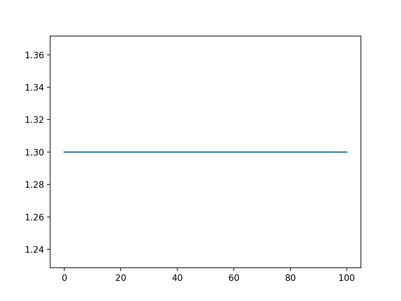
Constant

power1d.geom.Constant(Q=101, amp=0)

Constant value continuum with amplitude amp.

Keyword arguments:

Q —- continuum size (int) (default: 101)

amp —- continuum value (float or int) (default 0)

Example:

import power1d

obj = power1d.geom.Constant(Q=101, amp=1.3)
obj.plot()

(Source code, png, hires.png, pdf)

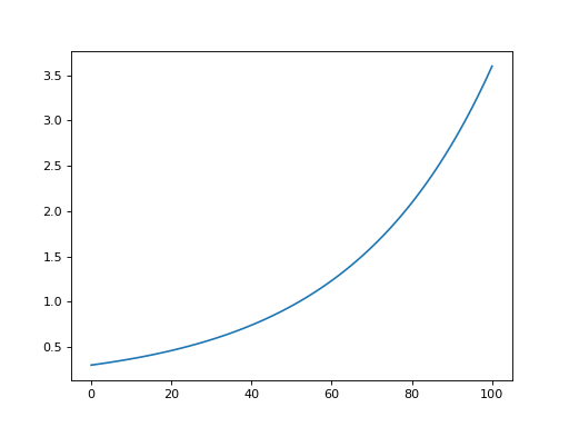
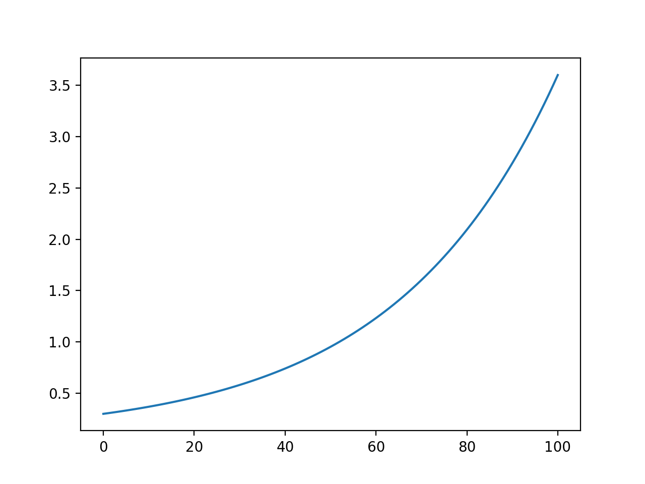
Exponential

power1d.geom.Exponential(Q=101, x0=0, x1=1, rate=1)

Exponentially increasing (or decreasing) continuum

Keyword arguments:

Q —- continuum size (int) (default: 101)

x0 —- value at starting continuum point (float or int) (default 0)

x1 —- value at ending continuum point (float or int) (default 1)

rate —- rate of exponential increase (float or int) (default 1)

Example:

import power1d

obj = power1d.geom.Exponential(Q=101, x0=0.3, x1=3.6, rate=2.8)
obj.plot()

(Source code, png, hires.png, pdf)

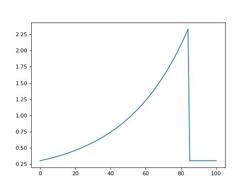
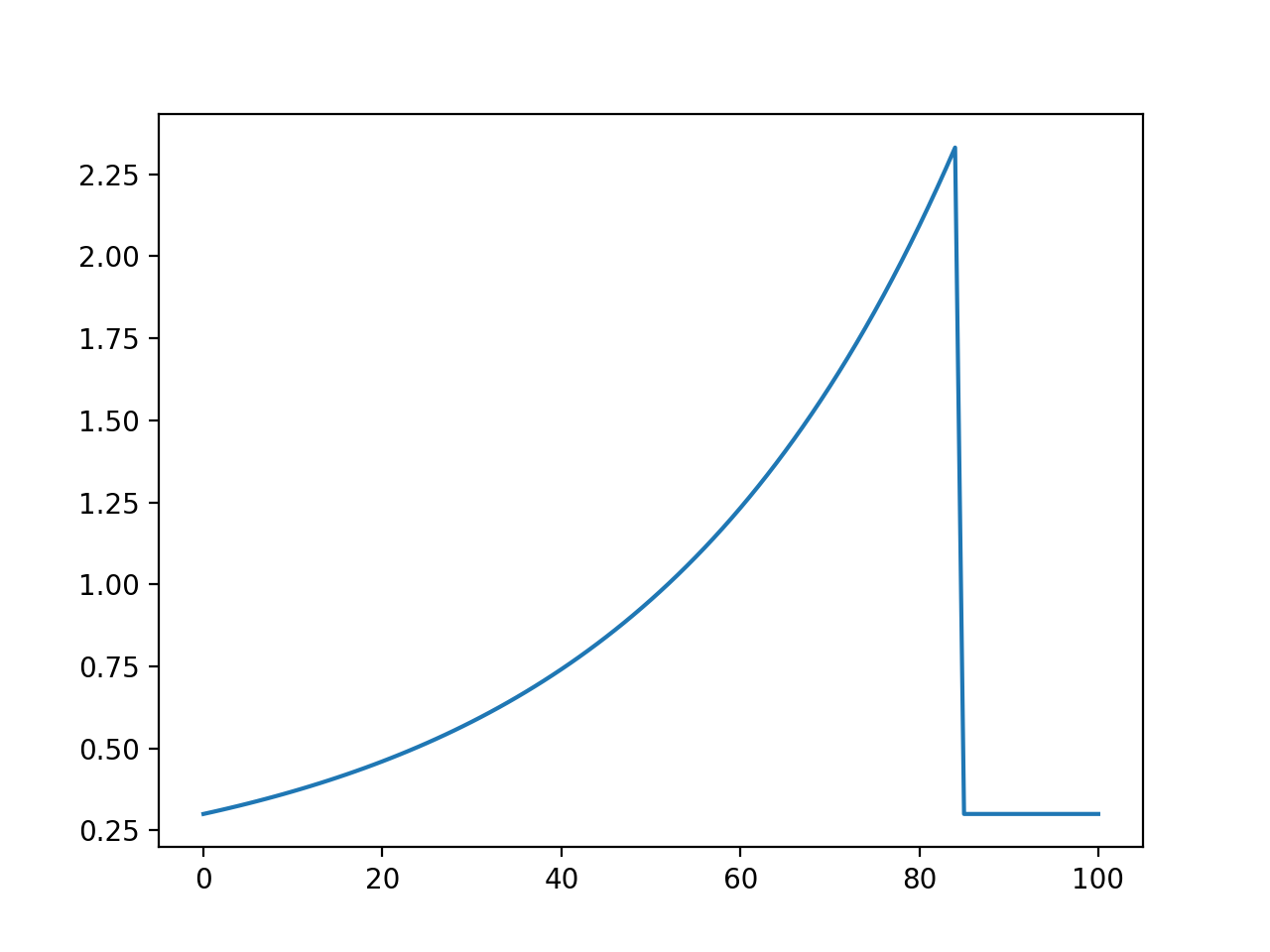
ExponentialSaw

power1d.geom.ExponentialSaw(Q=101, x0=0, x1=1, rate=1, cutoff=70)

Exponentially increasing (or decreasing) continuum with a saw cutoff

Keyword arguments:

Q —- continuum size (int) (default: 101)

x0 —- value at starting continuum point (float or int) (default 0)

x1 —- value at ending continuum point (float or int) (default 1)

rate —- rate of exponential increase (float or int) (default 1)

cutoff —- continuum point at which the continuum returns to x0 (int) (default 70)

Example:

import power1d

obj = power1d.geom.ExponentialSaw(Q=101, x0=0.3, x1=3.6, rate=2.8, cutoff=85)
obj.plot()

(Source code, png, hires.png, pdf)

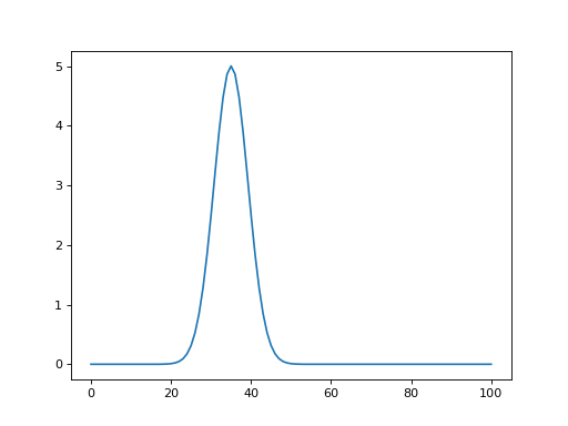
GaussianPulse

power1d.geom.GaussianPulse(Q=101, q=50, fwhm=None, sigma=None, amp=1)

A Gaussian pulse at a particular continuum location.

NOTE: one of fwhm and sigma must be specified, and the other must be None.

Keyword arguments:

Q —- continuum size (int) (default: 101)

q —- pulse center (int) (default 50)

fwhm —- pulse’s full-width-at-half-maximum (float or int) (default None)

sigma —- pulse’s standard deviation (float or int) (default None)

amp —- pulse amplitude

Example:

import power1d

obj = power1d.geom.GaussianPulse( Q=101, q=35, fwhm=10, amp=5 )
obj.plot()

(Source code, png, hires.png, pdf)

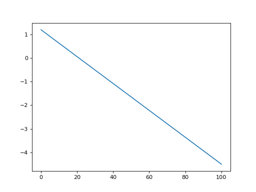
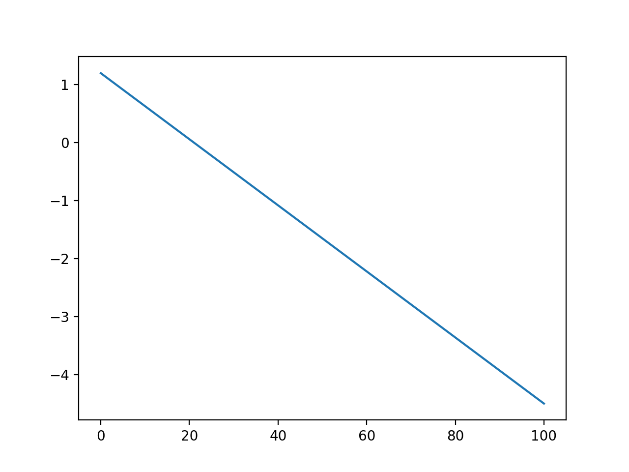
Linear

power1d.geom.Linear(Q=101, x0=0, x1=None, slope=None)

Linearly increasing (or decreasing) continuum

NOTE: one of x1 and slope must be specified, and the other must be None.

Keyword arguments:

Q —- continuum size (int) (default: 101)

x0 —- value at starting continuum point (float or int) (default 0)

x1 —- value at ending continuum point (float or int) (default None)

slope —- rate of linear increase (float or int) (default None)

Example:

import power1d

obj = power1d.geom.Linear( Q=101, x0=1.2, x1=-4.5 )
obj.plot()

(Source code, png, hires.png, pdf)

Null

power1d.geom.Null(Q=101)

Null continuum. This is equivalent to a constant continuum with amp=0

Keyword arguments:

Q —- continuum size (int) (default: 101)

Example:

import power1d

obj = power1d.geom.Null( Q=101 )
obj.plot()

(Source code, png, hires.png, pdf)

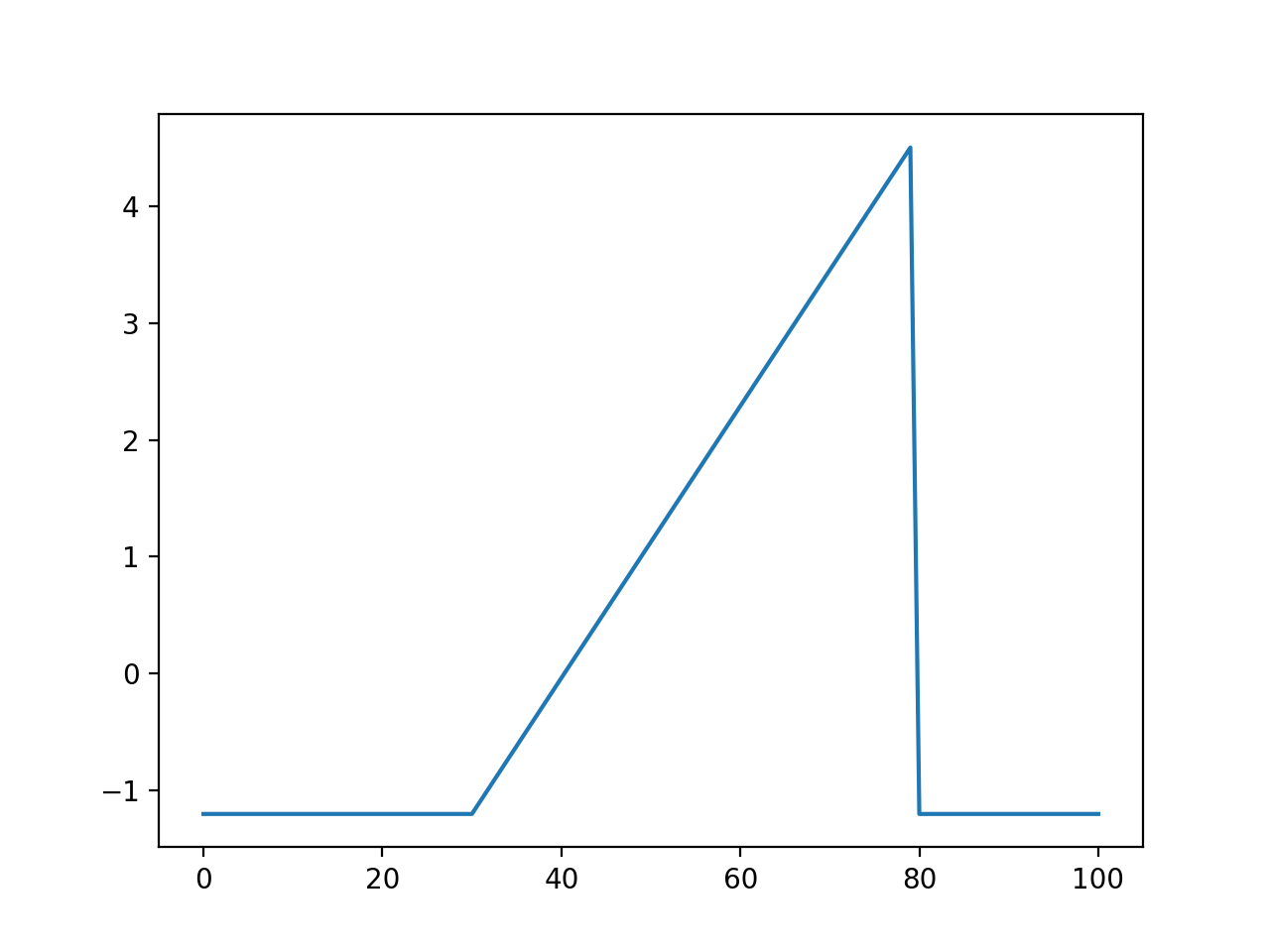
SawPulse

power1d.geom.SawPulse(Q=101, q0=50, q1=75, x0=0, x1=1)

Linearly increasing (or decreasing) continuum, cut-off at a particular point

Keyword arguments:

Q —- continuum size (int) (default: 101)

q0 —- continuum point at which the saw starts (int) (default 50)

q1 —- continuum point at which the saw end (int) (default 75)

x0 —- value at start point (float or int) (default 0)

x1 —- value at end point (float or int) (default 1)

Example:

import power1d

obj = power1d.geom.SawPulse( Q=101, q0=30, q1=80, x0=-1.2, x1=4.5 )
obj.plot()

(Source code, png, hires.png, pdf)

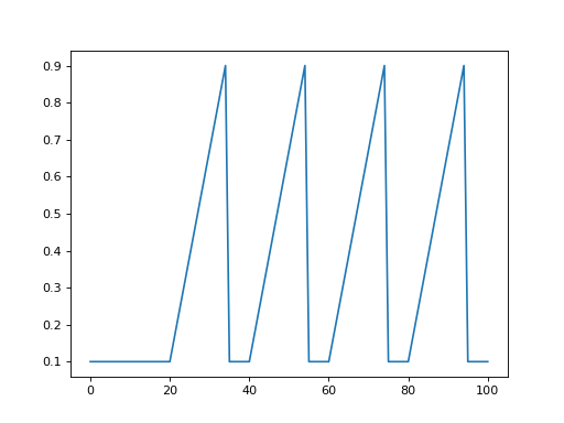
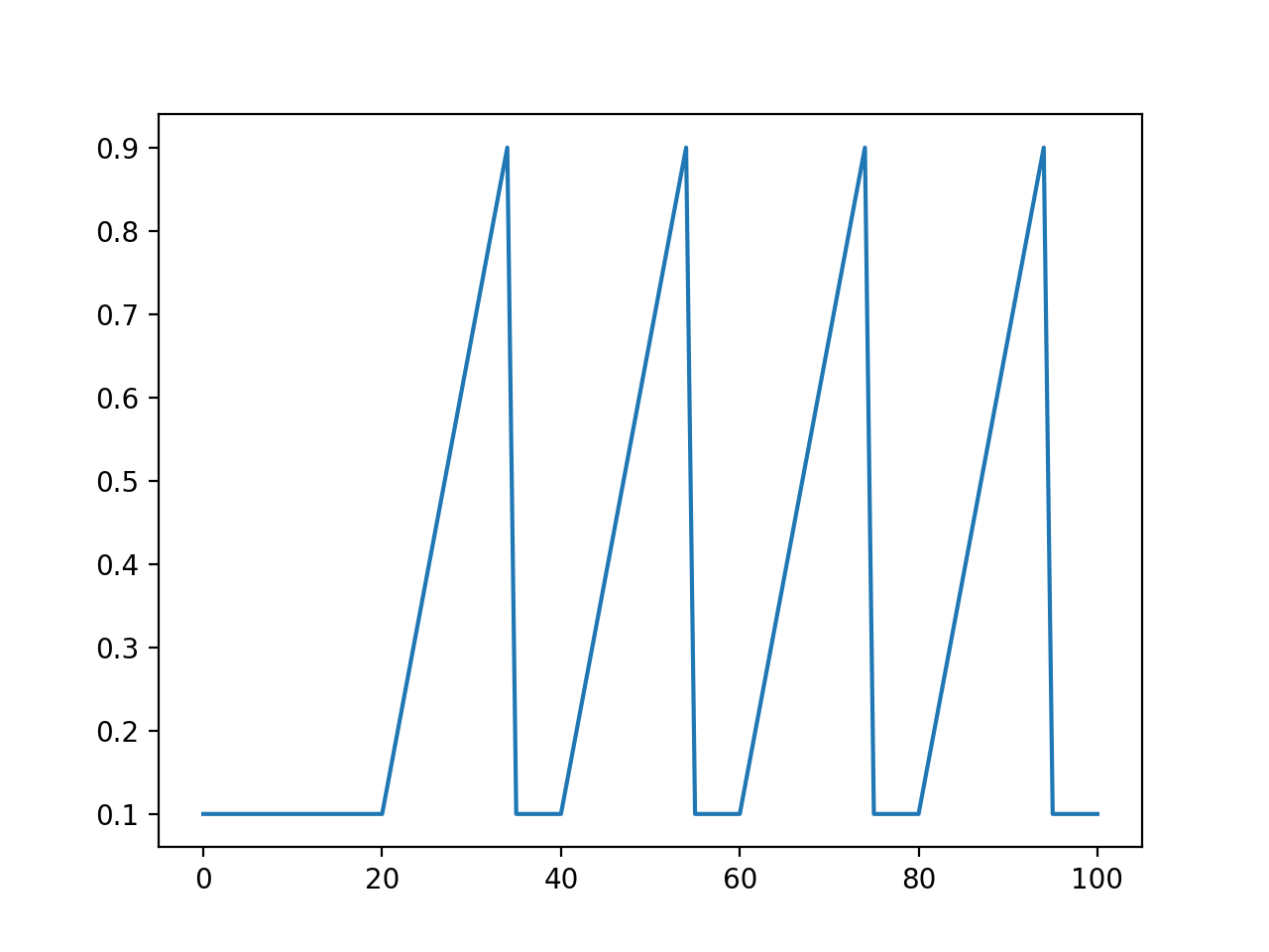
SawTooth

power1d.geom.SawTooth(Q=101, q0=50, q1=75, x0=0, x1=1, dq=0)

Repeating saw pattern.

Keyword arguments:

Q —- continuum size (int) (default: 101)

q0 —- continuum point at which the saw starts (int) (default 50)

q1 —- continuum point at which the saw ends (int) (default 75)

x0 —- value at start point (float or int) (default 0)

x1 —- value at end point (float or int) (default 1)

dq —- inter-tooth distance (int) (default 0)

Example:

import power1d

obj = power1d.geom.SawTooth( Q=101, q0=20, q1=35, x0=0.1, x1=0.9, dq=5 )
obj.plot()

(Source code, png, hires.png, pdf)

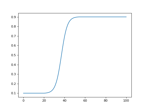
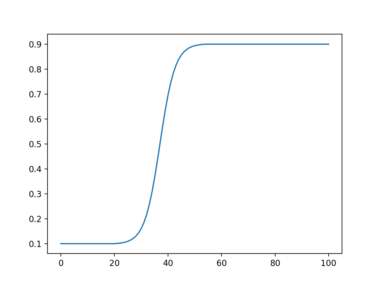
Sigmoid

power1d.geom.Sigmoid(Q=101, q0=50, q1=75, x0=0, x1=1)

Sigmoidal step pulse

Keyword arguments:

Q —- continuum size (int) (default: 101)

q0 —- continuum point at which the step starts (int) (default 50)

q1 —- continuum point at which the step ends (int) (default 75)

x0 —- value at start point (float or int) (default 0)

x1 —- value at end point (float or int) (default 1)

Example:

import power1d

obj = power1d.geom.Sigmoid( Q=101, q0=20, q1=55, x0=0.1, x1=0.9 )
obj.plot()

(Source code, png, hires.png, pdf)

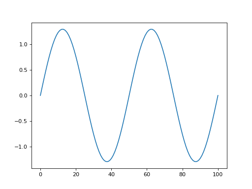
Sinusoid

power1d.geom.Sinusoid(Q=101, q0=0, amp=1, hz=1)

Repeating sinusoidal wave

Keyword arguments:

Q —- continuum size (int) (default: 101)

q0 —- continuum point at which phase is zero (int) (default 0)

amp —- amplitude (float or int) (default 1)

hz —- frequency relative to continuum size (float or int) (default 1)

Example:

import power1d

obj = power1d.geom.Sinusoid( Q=101, q0=0, amp=1.3, hz=2 )
obj.plot()

(Source code, png, hires.png, pdf)

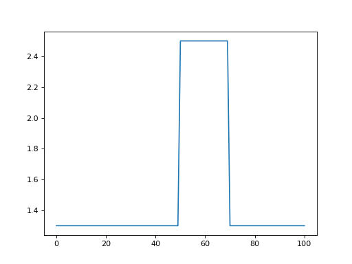
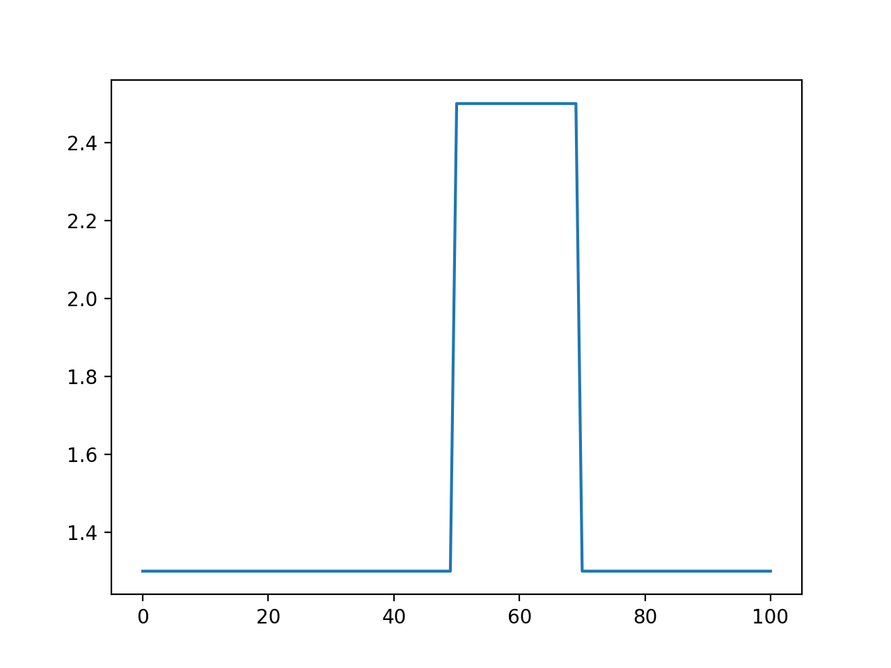
SquarePulse

power1d.geom.SquarePulse(Q=101, q0=50, q1=75, x0=0, x1=1)

Square pulse

Keyword arguments:

Q —- continuum size (int) (default: 101)

q0 —- continuum point at which pulse starts (int) (default 50)

q1 —- continuum point at which pulse ends (int) (default 75)

x0 —- starting value (int or float) (default 0)

x1 —- pulse height (int or float) (default 1)

Example:

import power1d

obj = power1d.geom.SquarePulse( Q=101, q0=50, q1=70, x0=1.3, x1=2.5 )
obj.plot()

(Source code, png, hires.png, pdf)

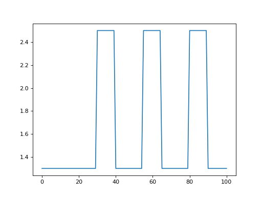
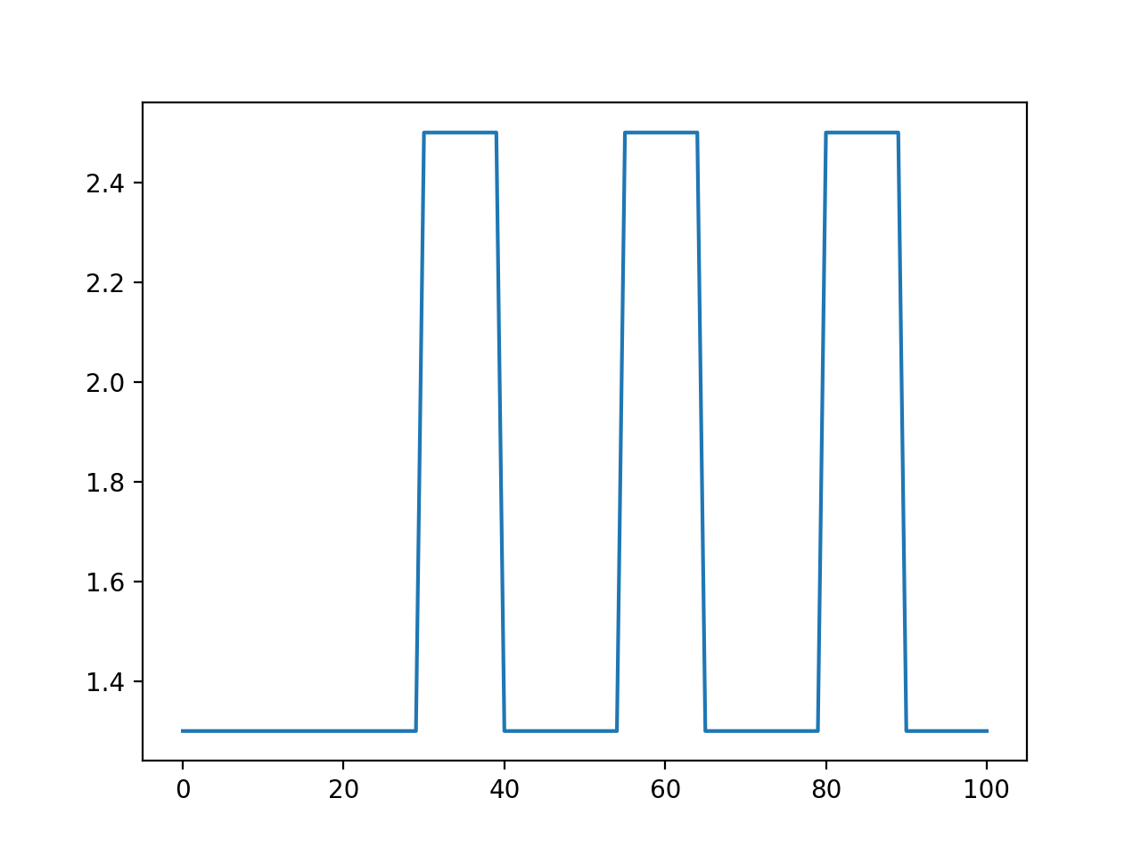
SquareTooth

power1d.geom.SquareTooth(Q=101, q0=10, q1=25, x0=0, x1=1, dq=5)

Repeating square pulses

Keyword arguments:

Q —- continuum size (int) (default: 101)

q0 —- continuum point at which pulse starts (int) (default 10)

q1 —- continuum point at which pulse ends (int) (default 25)

x0 —- starting value (int or float) (default 0)

x1 —- pulse height (int or float) (default 1)

dq —- inter-tooth distance (int) (default 5)

Example:

import power1d

obj = power1d.geom.SquareTooth( Q=101, q0=30, q1=40, x0=1.3, x1=2.5, dq=15 )
obj.plot()

(Source code, png, hires.png, pdf)

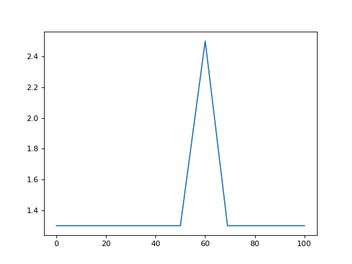
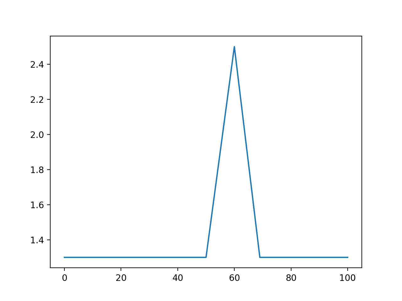
TrianglePulse

power1d.geom.TrianglePulse(Q=101, q0=50, q1=75, x0=0, x1=1)

Triangular pulse

Keyword arguments:

Q —- continuum size (int) (default: 101)

q0 —- continuum point at which pulse starts (int) (default 50)

q1 —- continuum point at which pulse ends (int) (default 75)

x0 —- starting value (int or float) (default 0)

x1 —- pulse height (int or float) (default 1)

Example:

import power1d

obj = power1d.geom.TrianglePulse( Q=101, q0=50, q1=70, x0=1.3, x1=2.5 )
obj.plot()

(Source code, png, hires.png, pdf)

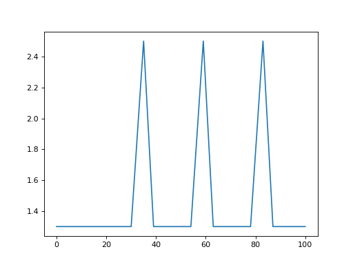
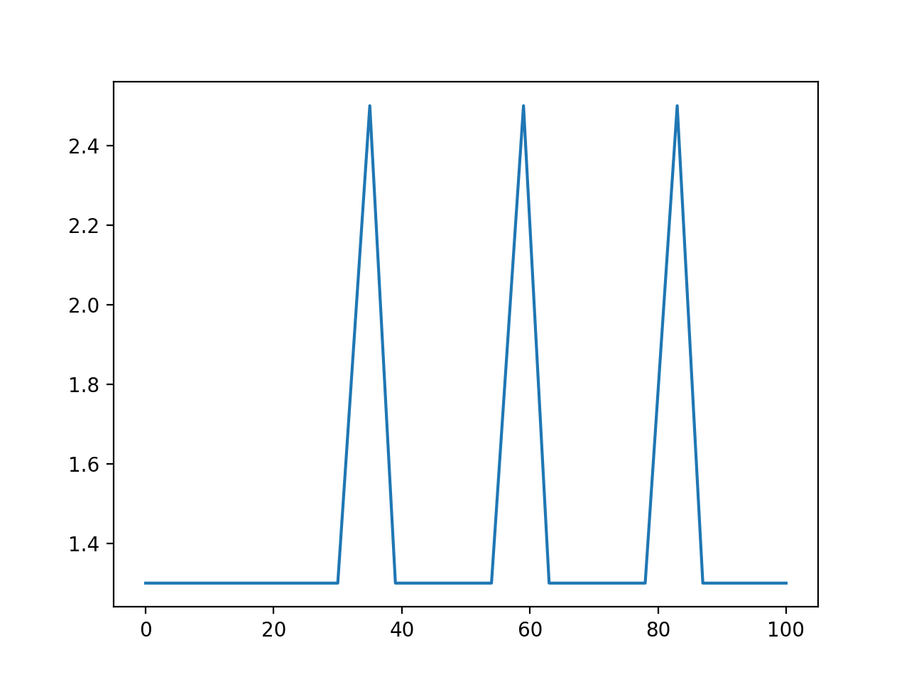
TriangleTooth

power1d.geom.TriangleTooth(Q=101, q0=50, q1=75, x0=0, x1=1, dq=20)

Repeating triangular pulses

Keyword arguments:

Q —- continuum size (int) (default: 101)

q0 —- continuum point at which pulse starts (int) (default 10)

q1 —- continuum point at which pulse ends (int) (default 25)

x0 —- starting value (int or float) (default 0)

x1 —- pulse height (int or float) (default 1)

dq —- inter-tooth distance (int) (default 5)

Example:

import power1d

obj = power1d.geom.TriangleTooth( Q=101, q0=30, q1=40, x0=1.3, x1=2.5, dq=15 )
obj.plot()

(Source code, png, hires.png, pdf)