Manual sample size calculation

Due to complexities such as the difference between omnibus and continuum-level powers, power1d does not directly support sample size calculation. Nevertheless, the sample sizes required to achieve certain powers can be estimated through iterative simulations as demonstrated below.

First build null and alternative models as follows:

import power1d

#(0) Create geometry and noise models:
J         = 5    # sample size
Q         = 101  # continuum size
q         = 65   # signal location
baseline  = power1d.geom.Null(Q=Q)
signal0   = power1d.geom.Null(Q=Q)
signal1   = power1d.geom.GaussianPulse(Q=101, q=q, amp=1.3, sigma=10)
noise     = power1d.noise.Gaussian(J=5, Q=101, sigma=1)

#(1) Create data sample models:
model0    = power1d.models.DataSample(baseline, signal0, noise, J=J)  #null
model1    = power1d.models.DataSample(baseline, signal1, noise, J=J)  #alternative

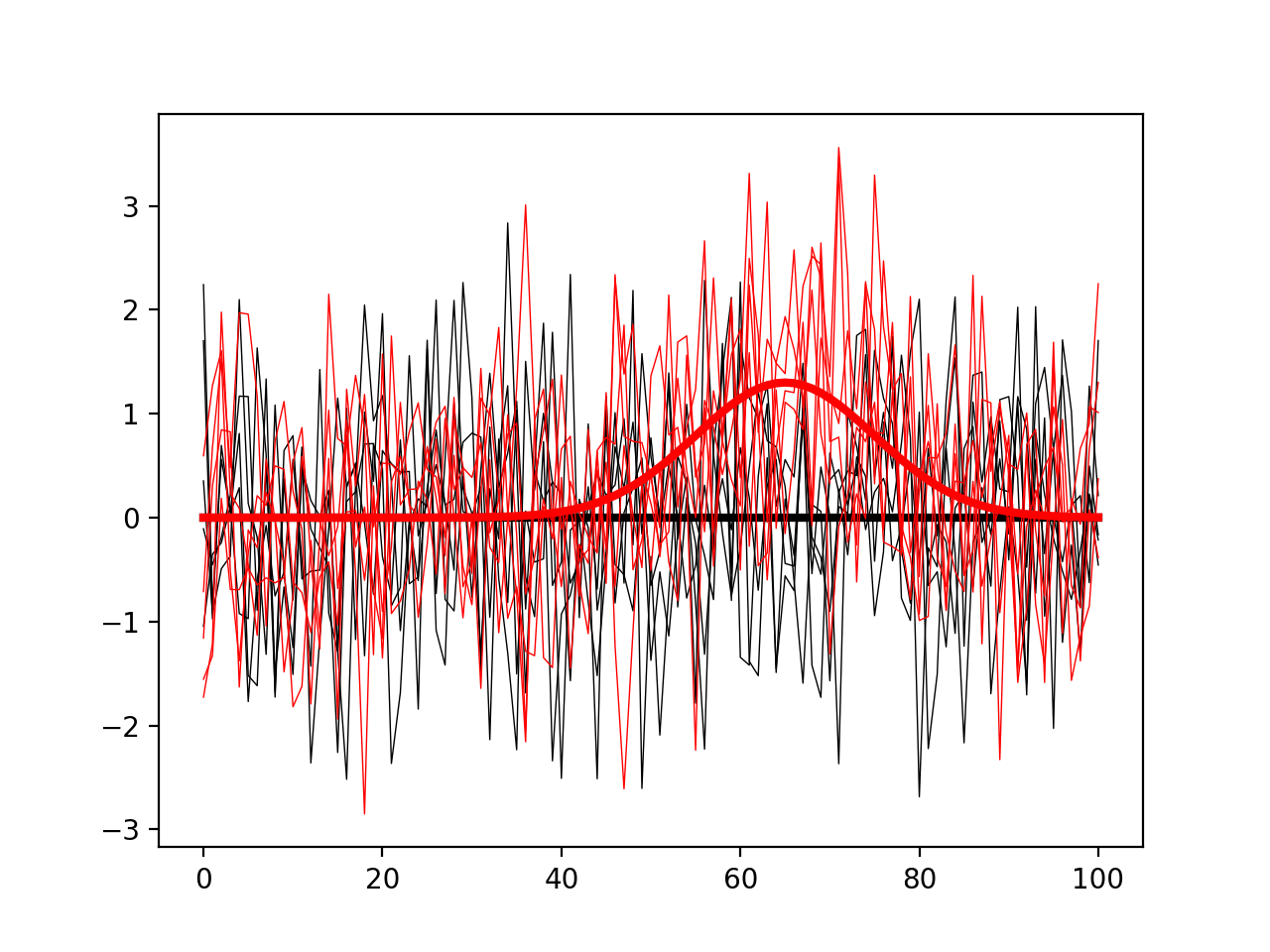
#(2) Visualize the models:
model0.plot( color='k' )
model1.plot( color='r' )

(Source code, png, hires.png, pdf)

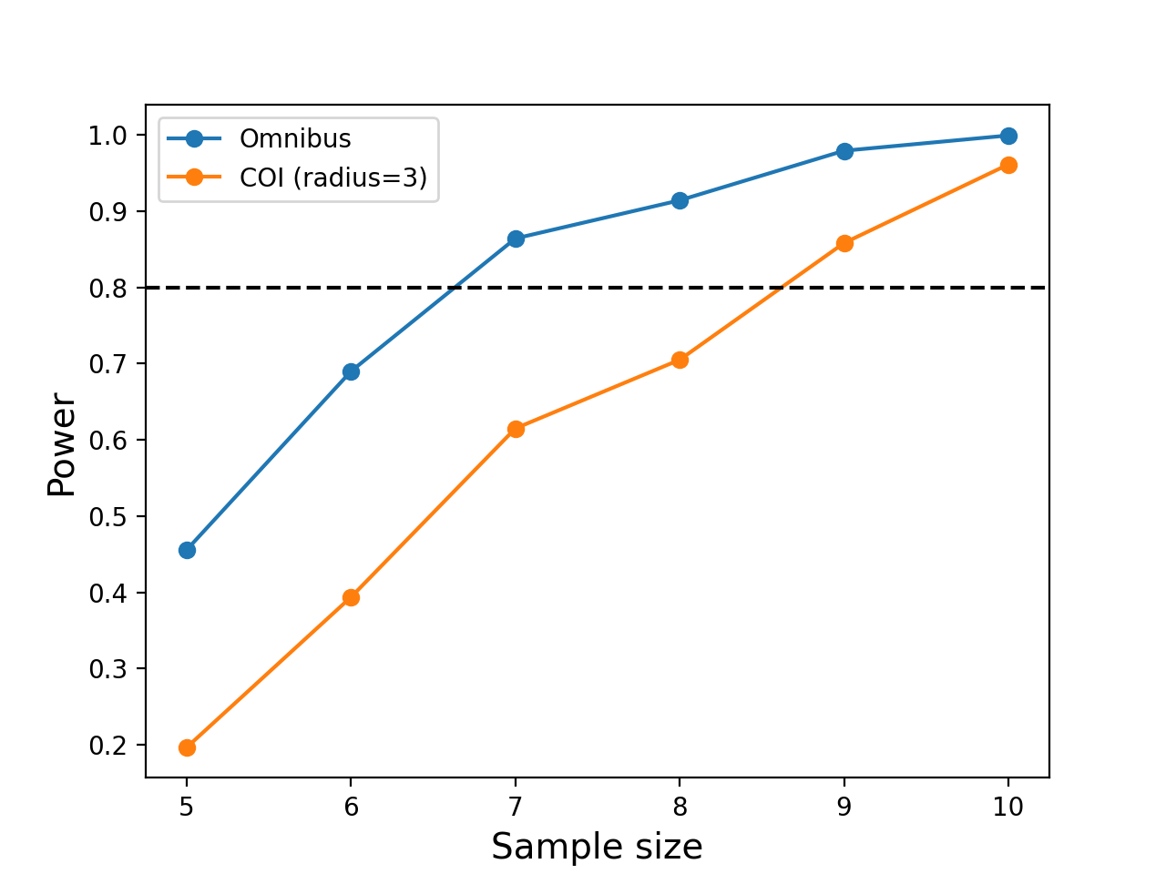
The goal is to compute the sample size J that will allow us to detect the modeled signal with a certain probability (usually 0.8). To do that iteratively simulate null and alternative experiments, and for each iteration store the power parameter of interest. In the script below both omnibus power and center-of-interest (COI) power (with a radius of 3) are saved for each iteration and plotted at the end.

import numpy as np
import matplotlib.pyplot as plt
import power1d

#(0) Create geometry and noise models:
J          = 5    # sample size
Q          = 101  # continuum size
q          = 65   # signal location
baseline   = power1d.geom.Null(Q=Q)
signal0    = power1d.geom.Null(Q=Q)
signal1    = power1d.geom.GaussianPulse(Q=101, q=q, amp=1.3, sigma=10)
noise      = power1d.noise.Gaussian(J=5, Q=101, sigma=1)

#(1) Create data sample models:
model0     = power1d.models.DataSample(baseline, signal0, noise, J=J)  #null
model1     = power1d.models.DataSample(baseline, signal1, noise, J=J)  #alternative

#(2) Iteratively simulate for a range of sample sizes:
np.random.seed(0)    #seed the random number generator
JJ         = [5, 6, 7, 8, 9, 10]  #sample sizes
tstat      = power1d.stats.t_1sample  #test statistic function
emodel0    = power1d.models.Experiment(model0, tstat) # null
emodel1    = power1d.models.Experiment(model1, tstat) # alternative
sim        = power1d.ExperimentSimulator(emodel0, emodel1)
### loop through the different sample sizes:
power_omni = []
power_coi  = []
coir       = 3
for J in JJ:
        emodel0.set_sample_size( J )
        emodel1.set_sample_size( J )
        results = sim.simulate( 1000 )
        results.set_coi( ( q , coir ) )  #create a COI at the signal location
        power_omni.append( results.p_reject1 )  #omnibus power
        power_coi.append( results.p_coi1[0] )   #coi power

#(3) Plot the results:
ax = plt.axes()
ax.plot(JJ, power_omni, 'o-', label='Omnibus')
ax.plot(JJ, power_coi,  'o-', label='COI (radius=%d)' %coir)
ax.axhline(0.8, color='k', linestyle='--')
ax.set_xlabel('Sample size', size=14)
ax.set_ylabel('Power', size=14)
ax.legend()
plt.show()

(Source code, png, hires.png, pdf)

These results suggest that the omnibus power reaches 0.8 for a sample size of J = 7 but that a sample size of J = 9 is needed for COI power of 0.8.

Note that the power vs. sample size curves are not smoothly increasing due to relatively small number of simulation iterations (1000). They will be more accurate for a larger number number of iterations, but the sample sizes required to achieve certain powers will likely not change dramatically.