Automated sample size calculation

(new in v.0.1.7)

Sample sizes can be estimated using the sample_size method of the ExperimentSimulator class. An example appears below.

Note that this procedure uses simple optimization to find the minimum sample size to meet the required power. Also see: manual power calculations.

import numpy as np
from matplotlib import pyplot as plt
import power1d


# create geometry and noise models:
J          = 5    # sample size
Q          = 101  # continuum size
q          = 65   # signal location
baseline   = power1d.geom.Null(Q=Q)
signal0    = power1d.geom.Null(Q=Q)
signal1    = power1d.geom.GaussianPulse(Q=101, q=q, amp=1.3, sigma=10)
noise      = power1d.noise.Gaussian(J=5, Q=101, sigma=1)


# create data sample models:
model0     = power1d.models.DataSample(baseline, signal0, noise, J=J)  #null
model1     = power1d.models.DataSample(baseline, signal1, noise, J=J)  #alternative


# iteratively simulate for a range of sample sizes:
np.random.seed(0)    #seed the random number generator
JJ         = [3, 4, 5, 6, 7, 8, 9, 10]  #sample sizes
tstat      = power1d.stats.t_1sample  #test statistic function
emodel0    = power1d.models.Experiment(model0, tstat) # null
emodel1    = power1d.models.Experiment(model1, tstat) # alternative
sim        = power1d.ExperimentSimulator(emodel0, emodel1)
results    = sim.sample_size(power=0.8, alpha=0.05, niter0=200, niter=2000, coi=dict(q=q, r=3))


# retrieve estimated sample size:
n          = results['nstar']
print( f'Estimate sample size = {n}' )


# plot:
plt.figure()
ax = plt.axes()
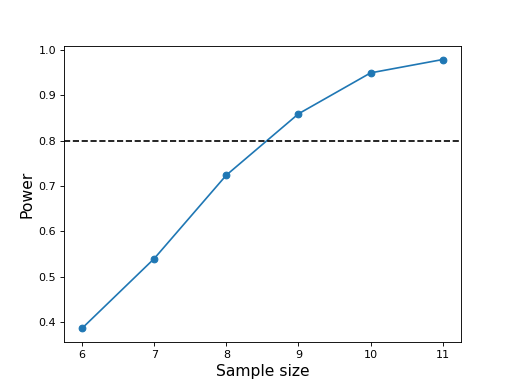
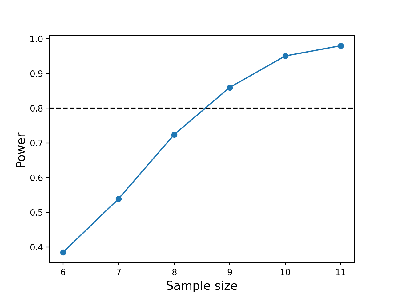
ax.plot( results['n'], results['p'], 'o-')
ax.axhline( results['target_power'] , color='k', linestyle='--')
ax.set_xlabel('Sample size', size=14)
ax.set_ylabel('Power', size=14)
plt.show()

(Source code, png, hires.png, pdf)