Parsing GUI results
The mwarp1d GUI saves all results in compressed NPZ format. This results file contains the original data, the warping parameters, and the warped data. Results are automatically saved every time the user updates a warp.
The results file can be parsed in one of two ways:
Using numpy.load
Using mwarp1d.loadnpz
The examples below consider the example results files:
./mwarp1d/examples/data/warps_Dorn2012_landmark.npz
./mwarp1d/examples/data/warps_Dorn2012_manual.npz
Using numpy.load (landmark mode)
The results file can be loaded using the usual NumPy approach. Let’s first check the variable names that are stored in landmark mode results.
In [1]:
import os
import numpy as np
from matplotlib import pyplot as plt
import mwarp1d


dirDATA  = mwarp1d.get_data_dir()
fnameNPZ = os.path.join(dirDATA, 'warps_Dorn2012_landmark.npz')

with np.load(fnameNPZ) as Z:
    for key in Z.keys():
        print(key)
mode
filename0
filename1
ydata_template
ydata_sources
ydata_sources_warped
landmarks_template
landmarks_sources
landmark_labels
These variables are:
mode — warping mode (“landmark” or “manual”)
filename0 — the name of the CSV data file (if any) imported into the GUI
filename1 — the name of the NPZ data file (originally specified in the GUI; this is not updated if the NPZ file is relocated)
ydata_template — template; a (Q,) array, where Q is the number of domain nodes
ydata_sources — original sources; a (J,Q) array, where J is the number of sources
ydata_sources_warped — warped sources; a (J,Q) array
landmarks_template — template landmarks, an (n,) array of integers, where n is the number of landmarks
landmarks_sources — source landmarks, a (J,n) array of integers
landmark_labels — landmark, an (n,) array of string labels, one per landmark
Let’s first check the mode and data array shapes:
In [2]:
with np.load(fnameNPZ) as Z:
    print( Z['mode'] )
    print( Z['ydata_template'].shape )
    print( Z['ydata_sources'].shape )
    print( Z['ydata_sources_warped'].shape )
landmark
(100,)
(7, 100)
(7, 100)
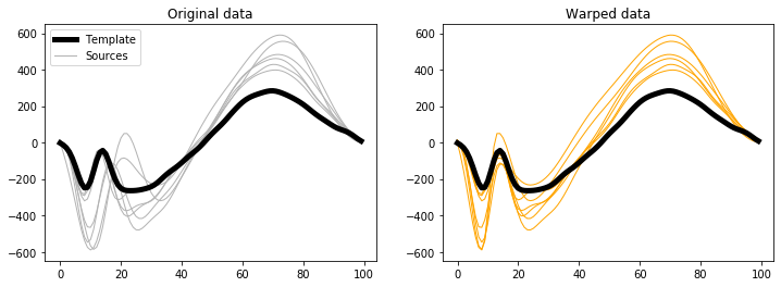
This implies that the data were warped in “landmark” mode, that there were 7 sources, each represented using 100 domain nodes.
Let’s next check the landmark array shapes:
In [3]:
with np.load(fnameNPZ) as Z:
    print( Z['landmarks_template'].shape )
    print( Z['landmarks_sources'].shape )
    print( Z['landmark_labels'].shape )
(4,)
(7, 4)
(4,)
This implies that 4 landmarks were used for each of the 7 sources.
The actual landmarks are:
In [4]:
with np.load(fnameNPZ) as Z:
    for key in ['landmarks_template', 'landmarks_sources', 'landmark_labels']:
        print('%s:' %key)
        print('%s' %Z[key])
        print()
landmarks_template:
[ 8 14 24 70]

landmarks_sources:
[[ 8 13 23 70]
 [ 8 14 25 70]
 [ 8 14 25 70]
 [10 17 27 72]
 [ 9 16 26 71]
 [10 21 32 72]
 [11 22 33 73]]

landmark_labels:
['C1' 'C2' 'C3' 'C']
The data can be visualized as follows:
In [5]:
with np.load(fnameNPZ) as Z:
    y0  = Z['ydata_template']
    y   = Z['ydata_sources']
    yw  = Z['ydata_sources_warped']


plt.figure( figsize=(12,4) )

ax  = plt.subplot(121)
h0  = ax.plot(y0,  'k', lw=5, zorder=1)[0]
h1  = ax.plot(y.T, '0.7', lw=1, zorder=0)[0]
ax.legend([h0,h1], ['Template','Sources'])
ax.set_title('Original data')

ax  = plt.subplot(122)
ax.plot(y0,  'k', lw=5, zorder=1)
ax.plot(yw.T, 'orange', lw=1, zorder=0)
ax.set_title('Warped data')


plt.show()
Using numpy.load (manual mode)
The variables saved for the manual warping mode are:
In [6]:
fnameNPZ = os.path.join(dirDATA, 'warps_Dorn2012_manual.npz')

with np.load(fnameNPZ) as Z:
    for key in Z.keys():
        print(key)
mode
filename0
filename1
ydata_template
ydata_sources
ydata_sources_warped
seqwarps
“seqwarps” is the only new variable; not also that the “landmarks*” variables do not appear in manual mode.
seqwarps — a (J,) array of objects, where each object is an array of sequential manual warp parameters.
In order to read seqwarps, the NPZ file must be loaded in “allow_pickle” mode as follows.
In [7]:
with np.load(fnameNPZ, allow_pickle=True) as Z:
    seqwarps = Z['seqwarps']

print(seqwarps)
[None None
 array([[0.03539823, 0.24285714, 0.162     , 0.162     ],
       [0.02758621, 0.27142857, 0.092     , 0.092     ]])
 array([[-0.24175824,  0.15714286,  0.396     ,  0.396     ],
       [ 0.09447005,  0.27142857,  0.07      ,  0.07      ],
       [-0.01442308,  0.7       ,  0.19      ,  0.19      ]])
 None
 array([[-0.32      ,  0.47142857,  0.99      ,  0.99      ],
       [ 0.12727273,  0.61428571,  0.476     ,  0.476     ],
       [-0.08      ,  0.18571429,  0.87      ,  0.        ]])
 array([[-0.35493827,  0.54285714,  0.962     ,  0.962     ],
       [ 0.05022831,  0.27142857,  0.328     ,  0.328     ],
       [ 0.14479638,  0.61428571,  0.774     ,  0.774     ],
       [-0.3       ,  0.        ,  0.04      ,  0.04      ]])]
Note that the elements of seqwarps are either None or an (m,4) array, where m is the number of warps applied to the given source, and 4 is the number of manual warp parameters (i.e., amp, center, head, tail).
For example, the sequential warp parameters for the third source can be retrieved using:
In [8]:
sw = seqwarps[2]

print(sw)
[[0.03539823 0.24285714 0.162      0.162     ]
 [0.02758621 0.27142857 0.092      0.092     ]]
These parameters could then be used in conjunction with the SequentialManualWarp class to reconstruct ydata_sources_warped.
However, if you wish to use these saved warping results (either landmark or manual mode results) to warp data, it is much easier to use mwarp1d.loadnpz as described below.
Using mwarp1d.loadnpz
The NPZ results files can alternatively be loaded using mwarp1d.loadnpz:
In [9]:
results = mwarp1d.loadnpz(fnameNPZ)

print(results)
MWarpResults
----- Overview -------------
    mode           = manual
    nsources       = 7
    nnodes         = 100
----- 1D Data -------------
    sources        = (7,100) array
    sources_warped = (7,100) array
    template       = (100,) array
Summary information is displayed, and all parameters can be accessed as attributes like this:
In [10]:
print( results.mode )
print( results.nsources )
print( results.nnodes )
print( results.sources.shape )
manual
7
100
(7, 100)
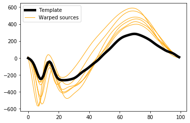
and visualized like this:
In [11]:
plt.figure()
ax  = plt.axes()
h0  = ax.plot(results.template,  'k', lw=5, zorder=1)[0]
h1  = ax.plot(results.sources_warped.T, 'orange', lw=1, zorder=0)[0]
ax.legend([h0,h1], ['Template','Warped sources'])
plt.show()
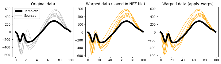
The most useful feature of this loadnpz procedure is the apply_warps method, which can be used to warp arbitrary data. For example, to reproduce the saved warped sources, simply submit the original sources to apply_warps like this:
In [12]:
y0 = results.template
y  = results.sources
yw = results.sources_warped

ywcheck = results.apply_warps( y )
Then compare the results:
In [13]:
plt.figure( figsize=(12,3) )

ax  = plt.subplot(131)
h0  = ax.plot(y0,  'k', lw=5, zorder=1)[0]
h1  = ax.plot(y.T, '0.7', lw=1, zorder=0)[0]
ax.legend([h0,h1], ['Template','Sources'])
ax.set_title('Original data')

ax  = plt.subplot(132)
ax.plot(y0,  'k', lw=5, zorder=1)
ax.plot(yw.T, 'orange', lw=1, zorder=0)
ax.set_title('Warped data (saved in NPZ file)')

ax  = plt.subplot(133)
ax.plot(y0,  'k', lw=5, zorder=1)
ax.plot(ywcheck.T, 'orange', lw=1, zorder=0)
ax.set_title('Warped data (apply_warps)')

plt.show()
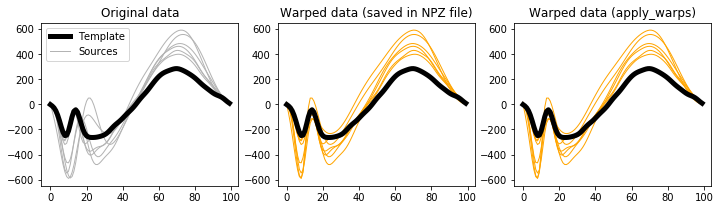
This apply_warps procedure can also be applied to landmark warps:
In [14]:
dirDATA  = mwarp1d.get_data_dir()
fnameNPZ = os.path.join(dirDATA, 'warps_Dorn2012_landmark.npz')
results  = mwarp1d.loadnpz(fnameNPZ)

y0       = results.template
y        = results.sources
yw       = results.sources_warped
ywcheck  = results.apply_warps( y )


plt.figure( figsize=(12,3) )

ax  = plt.subplot(131)
h0  = ax.plot(y0,  'k', lw=5, zorder=1)[0]
h1  = ax.plot(y.T, '0.7', lw=1, zorder=0)[0]
ax.legend([h0,h1], ['Template','Sources'])
ax.set_title('Original data')

ax  = plt.subplot(132)
ax.plot(y0,  'k', lw=5, zorder=1)
ax.plot(yw.T, 'orange', lw=1, zorder=0)
ax.set_title('Warped data (saved in NPZ file)')

ax  = plt.subplot(133)
ax.plot(y0,  'k', lw=5, zorder=1)
ax.plot(ywcheck.T, 'orange', lw=1, zorder=0)
ax.set_title('Warped data (apply_warps)')

plt.show()
This feature is particularly useful when you want to apply warps to multivariate 1D data, as demonstrated in Apply GUI warps