Application
This section describes how RFT can be used to make statistical inferences regarding sets of smooth 1D fields.
Example dataset
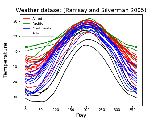
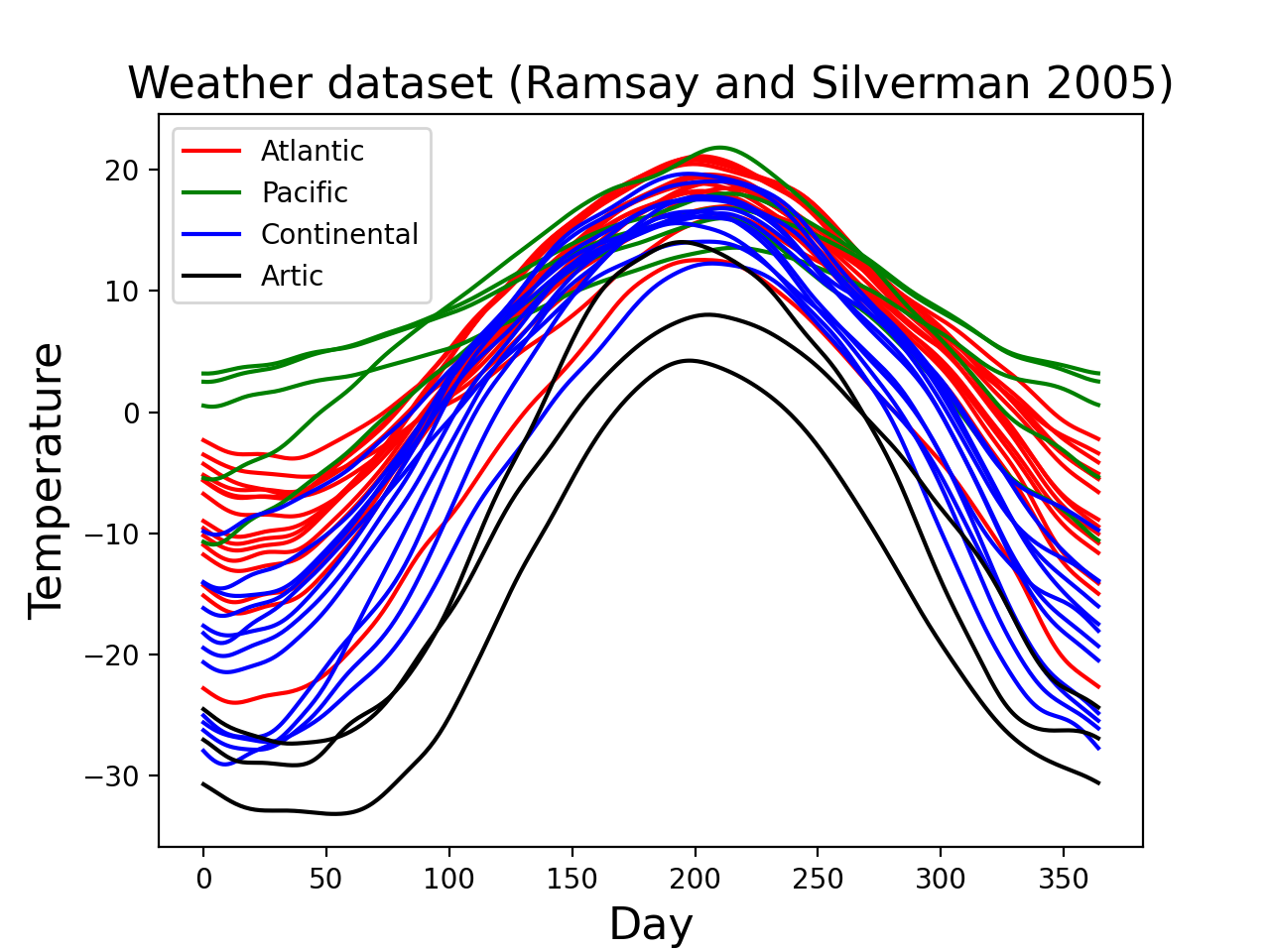
Consider the “weather” dataset depicted in the figure below. This dataset is publicly available at http://www.psych.mcgill.ca/misc/fda/downloads/FDAfuns/Matlab in the “weather.zip” folder. The dataset is described in detail here: http://www.psych.mcgill.ca/misc/fda/ex-weather-a1.html and also in the book:
Ramsay JO, Silverman BW (2005). Functional Data Analysis (Second Edition), Springer, New York. (see Chapter 13: “Modelling functional responses with multivariate covariates”)
These are daily temperature data from four different regions of Canada. Each field represents the recordings at one of 35 separate weather stations.
(Source code, png, hires.png, pdf)

Parametric inference using RFT
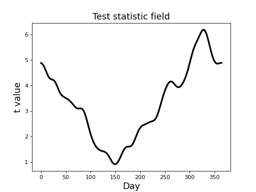
For simplicity’s let’s consider just two regions: Atlantic and Continental (the regions with the most observations: 15 and 12, respectively). If the data for these two regions are stored in variables “yA” and “yB”, respectively, where each variable is a NumPy array with shape (nResponses, 365), then then the two-sample t statistic field computed as follows:
>>> nA,nB = 15,12  #sample sizes
>>> mA,mB = yA.mean(axis=0), yB.mean(axis=0)  #means
>>> sA,sB = yA.std(ddof=1, axis=0), yB.std(ddof=1, axis=0)  #standard deviations
>>> s = np.sqrt( ((nA-1)*sA*sA + (nB-1)*sB*sB) / (nA + nB - 2) )  #pooled standard deviation
>>> t = (mA-mB) / ( s *np.sqrt(1.0/nA + 1.0/nB))  #t field
Note
For simplicity this t field calculation assumes equal variance, but field-level non-spherecity corrections exist (Friston et al. 2007).
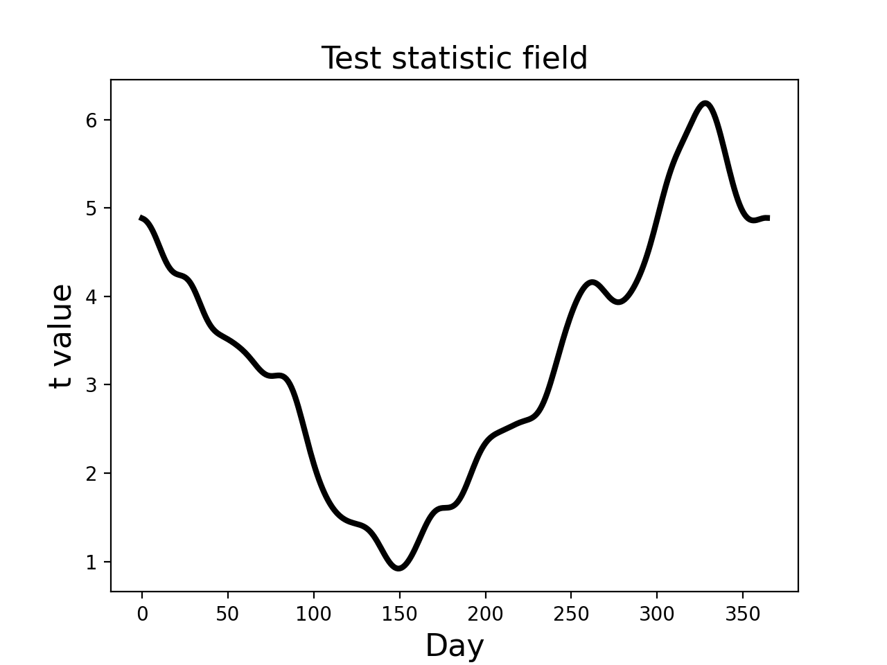
The resulting t field (depicted in the figure below) suggests that temperature differences between the Atlantic and Continental regions are largest in the winter months, reflecting the same trend in the raw fields (above).
(Source code, png, hires.png, pdf)
From a classical hypothesis testing perspective the relevant question is this:
What height would Gaussian fields (with the same FWHM as the model residuals) reach with a probability of
?
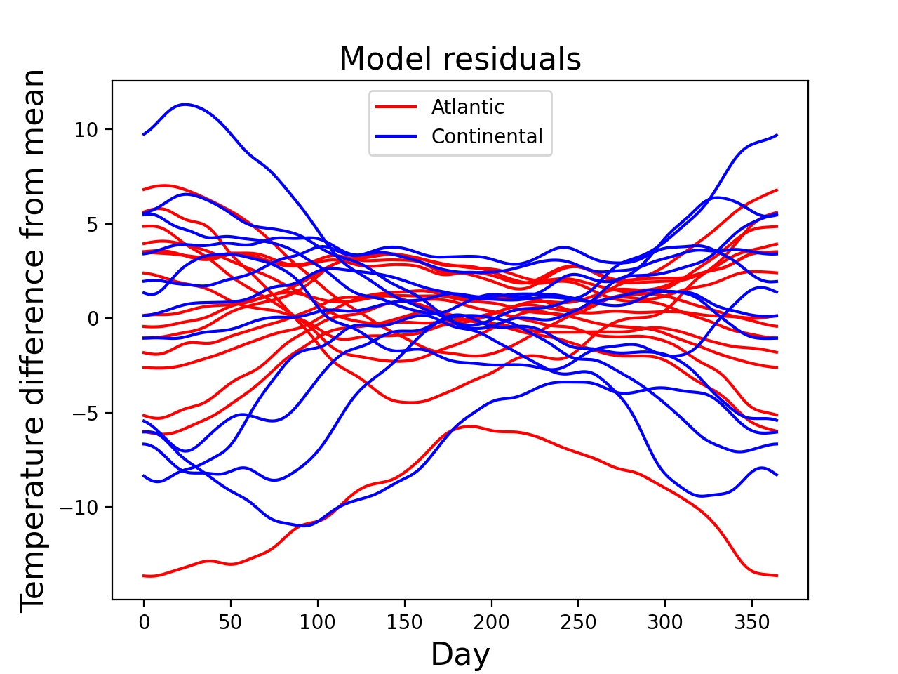
To answer that question we need to first compute the model residuals, in this case by simply subtracting field means from the original fields:
>>> residualsA,residualsB = yA-mA, yB-mB #residual fields
These residuals may be regarded as Gaussian random fields, and they look like this:
(Source code, png, hires.png, pdf)
Next we estimate the field smoothness using all residuals as follows:
>>> residuals = np.vstack([rA,rB]) #all residual fields; shape=(27,365)
>>> FWHM = rft1d.geom.estimate_fwhm(residuals) #yields #135.7
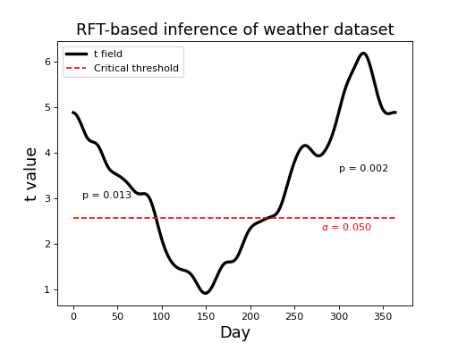
Since we know the FWHM (135.7) and we know the field length (365 nodes), we have all the parameters we need to conduct parametric inference:
>>> alpha = 0.05
>>> df = nA + nB - 2  #degrees of freedom
>>> nNodes = 365
>>> tstar = rft1d.t.isf(alpha, df, nNodes, FWHM) #inverse survival function
This yields a critical threhsold of 2.566, as depicted in the figure
below. Since the test statistic field exceeds the critical threshold
we would reject the null hypothesis at = 0.05.
To supplement the main null hypothesis rejection, we can next conduct set-level and cluster-level inference. For both we need the upcrossing extents:
>>> calc = rft1d.geom.ClusterMetricCalculator()
>>> k_nodes = calc.cluster_extents(t, tstar, interp=True)
>>> k_resels = [kk/FWHM for kk in k_nodes]
>>> c = len(k) #number of upcrossings
Set-level inference requires c and the smallest value from k_resels:
>>> rftcalc = rft1d.prob.RFTCalculator(STAT='T', df=(1,df), nodes=nNodes, FWHM=FWHM)
>>> k_min = min(k_resels)
>>> Pset = rftcalc.p.set(c, k_min, tstar)
The resulting p value (8.244e-05) represents the probability that Gaussian fields would produce at least c upcrossings with a minimum extent of k_min when thresholded at tstar. Since this probability pertains to the entire excursion set, and thus in this case to the whole year, we cannot use this result to make conclusion about particular parts of the year. For that we can use cluster-level inference:
>>> Pcluster = [rftcalc.p.cluster(kk, tstar) for kk in k_resels]
This yields the p values depicted in the figure below (0.013 and 0.002). These represent the probability that Gaussian fields would produce an upcrossing of extent kk when thresholded at tstar.
(Source code, png, hires.png, pdf)
Note
If an upcrossing just touches the critical threshold, its p value is (by defintion).
A non-parametric approach described below yields nearly identical results, suggesting that the parametric approach’s assumption of Gaussian field variance is a reasonably good one.
Note that the results above separate the upcrossings which touch the field border. It is probably more appropriate to regard the field as circular (since the first day of the new year follows the last day of the previous year), and thus to regard the upcrossings as connected. This can be achieved easily using the keyword wrap to rft1d procedures as described below
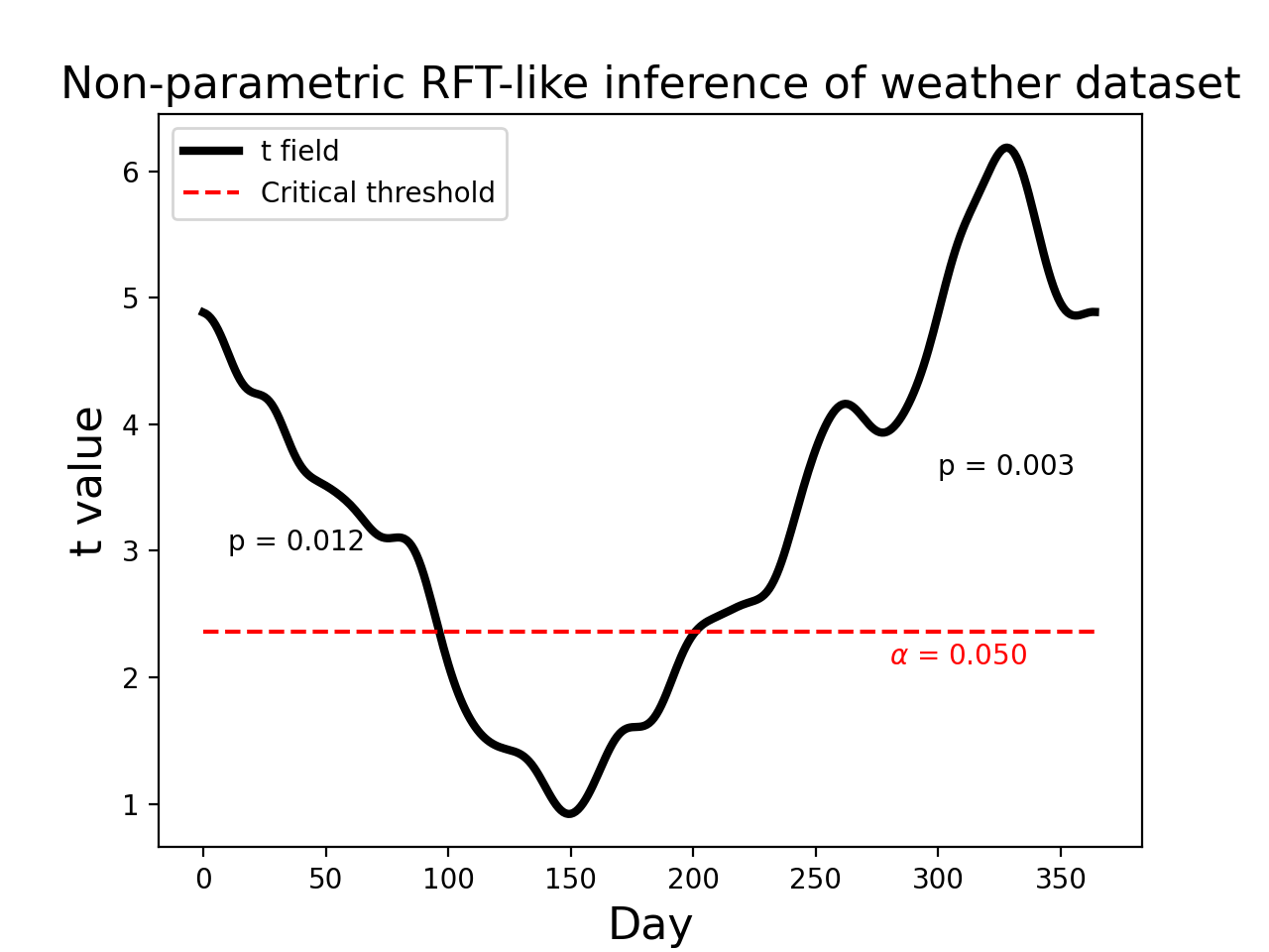
Non-parametric inference
A conceptually identical non-parametric permutation approach has been described by Nichols and Holmes (2002). It proceeds the same as typical permutation tests, with the minor exception that it constructs separate empirical distributions: one for the field maximum, and following that: one for upcrossings. The approach can be summarized as follows:
Randomly permute the labels
Compute the test statistic field based on the new labels.
Extract the field maximum (z_max).
Repeat (1)–(3) until all permutations have been exhausted or until the z_max distribution is reasonably stable.
Extract the critical test statistic (z_star) from the z_max distribution.
Repeat (1)–(4), this time extracting the maximum upcrossing extent (k_max) at threshold z_star for each permutation.
Compute upcrossing-specific p values based on the empirical k_max distribution.
The results are depicted in the figure below. The non-parametric critical threshold (2.359) is somewhat lower than the parametric threshold (2.566), but the upcrossing p values are essentially identical. Click on “source code” below to see coding details.
(Source code, png, hires.png, pdf)

Note
The non-parametric approach of offers a number of other advantages, such as estimated variance field smoothing, which can improve statistical power ((Nichols and Holmes, 2002)). The purpose here was to demonstrate only that, like the 0D case, complimentary non-parametric approaches also exist for the 1D case.
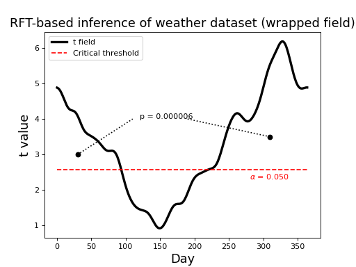
Field wrapping
Since this dataset is cyclical (i.e. after 31 December comes 1 Jan) inference is more appropriately conducted by wrapping the upcrossing as indicated in the figure below. Notice that there is just one p value, corresponding to the single (wrapped) upcrossing. Its p value is much lower because its extent is much greater.
(Source code, png, hires.png, pdf)