power1d.models
High-level classes for assembling data models and simulating experiments.
Below attributes and methods can be distinguished as follows:
attribute names are followed by “= None”
method names are followed by “( )” with arguments inside the parentheses, and all methods also have code snippets attached.
datasample_from_array
- power1d.models.datasample_from_array(y)
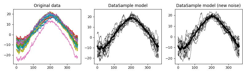
Convenience function for creating a data sample from a set of of 1D observations.
The input array must have a shape (J,Q) where:
J = number of observations
Q = number of continuum nodes
WARNING! “datasample_from_array” uses a relatively simple SmoothGaussian noise model, and this may NOT embody all features of real, experimental noise. In this case more complex noise modeling (e.g. Additive, Mixture) may be required. Refer to the noise module for more details.
import numpy as np
import matplotlib.pyplot as plt
import power1d

y        = power1d.data.weather()['Atlantic']
model    = power1d.models.datasample_from_array( y )

plt.close('all')
fig,axs = plt.subplots(1, 3, figsize=(10,3), tight_layout=True)
axs[0].plot( y.T )
np.random.seed(0)
model.random()
model.plot( ax=axs[1])
model.random()
model.plot( ax=axs[2] )
labels  = 'Original data', 'DataSample model', 'DataSample model (new noise)'
[ax.set_title(s) for ax,s in zip(axs,labels)]
plt.show()
(Source code, png, hires.png, pdf)
DataSample
- class power1d.models.DataSample(baseline, signal, noise, J=8, regressor=None)
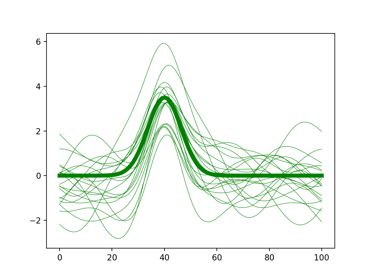
Data Sample model.
Arguments:
baseline —- a power1d.geom object representing the sample datum
signal —- a power1d.geom object representing the sample signal
noise —- a power1d.noise object representing the sample noise
J —- sample size (int, default 8)
regressor —- an optional regressor that will scale the signal across the J observations (length-J numpy array)
Example:
import matplotlib.pyplot as plt
import power1d

J        = 20
Q        = 101
baseline = power1d.geom.Null( Q=Q )
signal   = power1d.geom.GaussianPulse( Q=Q, q=40, fwhm=15, amp=3.5 )
noise    = power1d.noise.SmoothGaussian( J=J, Q=Q, mu=0, sigma=1.0, fwhm=20 )
model    = power1d.models.DataSample(baseline, signal, noise, J=J)
plt.close('all')
model.plot(color="g", lw=5)
(Source code, png, hires.png, pdf)

- J
sample size
- Q
continuum size
- baseline
baseline model
- get_baseline()
Return the DataSample’s baseline object
- get_noise()
Return the DataSample’s noise object
- get_signal()
Return the DataSample’s signal object
- link(other)
Link noise to another DataSample object so that the linked object’s noise is equivalent to master object’s noise.
- noise
noise model
- plot(ax=None, with_noise=True, color='k', lw=3, q=None)
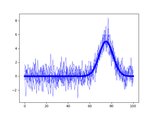
Plot an instantaneous representation of the DataSample
Arguments:
ax —- pyplot axes object (default None)
with_noise —- whether or not to plot the noise (bool, default True)
color —- a matplotlib color for all lines (baseline, signal and noise) (default “k” – black)
lw —- linewidth for the signal (int, default 3)
q —- optional continuum position values (length-Q array of monotonically increasing values) (default None)
Example:
import matplotlib.pyplot as plt
import power1d

J        = 8
Q        = 101
baseline = power1d.geom.Null( Q=Q )
signal   = power1d.geom.GaussianPulse( Q=Q, q=75, fwhm=15, amp=5.0 )
noise    = power1d.noise.Gaussian( J=J, Q=Q, mu=0, sigma=1.0 )
model    = power1d.models.DataSample(baseline, signal, noise, J=J)
plt.close('all')
model.plot(color="b", lw=5)
(Source code, png, hires.png, pdf)

- random(subtract_baseline=False)
Generate a random data sample based on the baseline, signal and noise models. The value will be stored in the “value” attribute.
- regressor
(J,) numpy array representing regressor
- set_baseline(baseline)
Change the DataSample’s baseline object
Arguments:
baseline —- a power1d.geom object representing the sample datum
- set_noise(noise)
Change the DataSample’s baseline object
Arguments:
baseline —- a power1d.noise object representing the sample datum
- set_regressor(x)
Set or change the DataSample’s regressor
Arguments:
x —- a length-J numpy array (float)
- set_sample_size(J)
Change the sample size
Arguments:
J —- sample size (positive int)
- set_signal(signal)
Change the DataSample’s signal object
Arguments:
signal —- a power1d.geom object representing the sample signal
- signal
signal model
Experiment
- class power1d.models.Experiment(data_sample_models, fn)
Experiment model.
Arguments:
data_sample_models —- a list of DataSample objects
fn —- a function for computing the test statistic (must accept a sequence of (J,Q) arrays and return a length-Q array representing the test statistic continuum). Standard test statistic functions are available in power1d.stats
Example:
import matplotlib.pyplot as plt
import power1d

J        = 10
Q        = 101
baseline = power1d.geom.Null( Q=Q )
signal0  = power1d.geom.Null( Q=Q )
signal1  = power1d.geom.GaussianPulse( Q=Q, q=40, fwhm=15, amp=3.5 )
noise    = power1d.noise.Gaussian( J=J, Q=Q, mu=0, sigma=1.0 )
model0   = power1d.models.DataSample(baseline, signal0, noise, J=J)
model1   = power1d.models.DataSample(baseline, signal1, noise, J=J)
emodel   = power1d.models.Experiment( [model0, model1], fn=power1d.stats.t_2sample )
plt.close('all')
emodel.plot()
(Source code, png, hires.png, pdf)
- Q
continuum length
- Z
output test statistic continua
- data_models
data models
- fn
test statistic function
- nmodels
number of data models
- plot(ax=None, with_noise=True, colors=None, q=None)
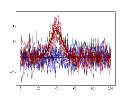
Plot an instantaneous representation of the Experiment model.
Arguments:
ax —- pyplot axes object (default None)
with_noise —- whether or not to plot the noise (bool, default True)
colors —- an optional sequence of matplotlib colors, one for each DataSample (default None)
q —- optional continuum position values (length-Q array of monotonically increasing values) (default None)
Example:
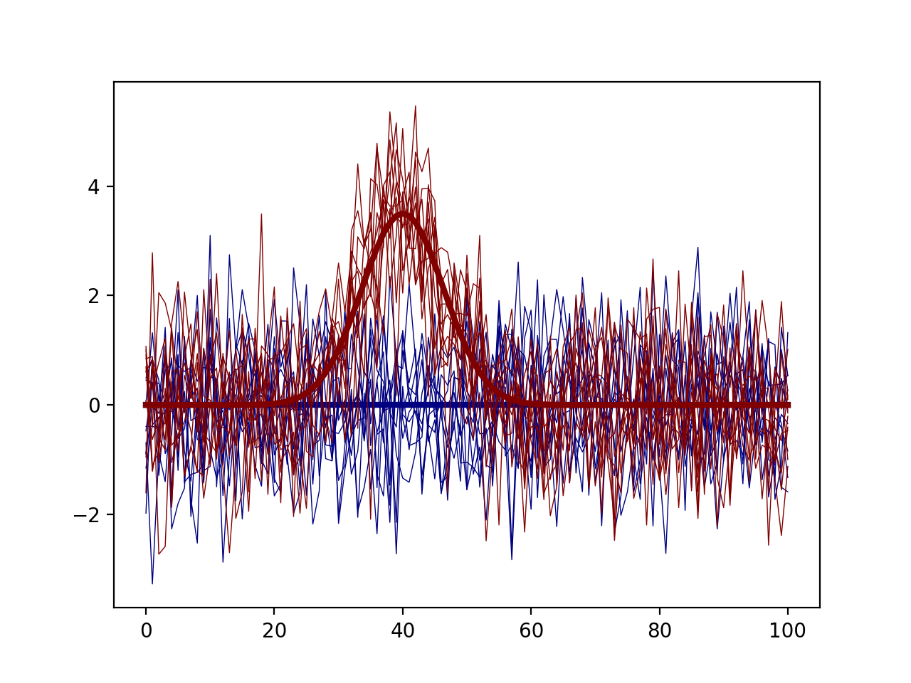
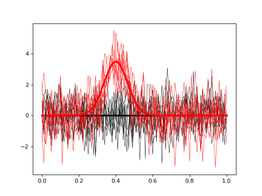
import numpy as np
import matplotlib.pyplot as plt
import power1d

J        = 8
Q        = 101
baseline = power1d.geom.Null( Q=Q )
signal0  = power1d.geom.Null( Q=Q )
signal1  = power1d.geom.GaussianPulse( Q=Q, q=40, fwhm=15, amp=3.5 )
noise    = power1d.noise.Gaussian( J=J, Q=Q, mu=0, sigma=1.0 )
model0   = power1d.models.DataSample(baseline, signal0, noise, J=J)
model1   = power1d.models.DataSample(baseline, signal1, noise, J=J)
emodel   = power1d.models.Experiment( [model0, model1], fn=power1d.stats.t_2sample )
plt.close('all')
emodel.plot( colors=("k", "r"), q=np.linspace(0, 1, Q) )
(Source code, png, hires.png, pdf)

- set_sample_size(JJ)
Change the sample sizes of the models
Arguments:
J —- sample size (positive int or list of positive int)
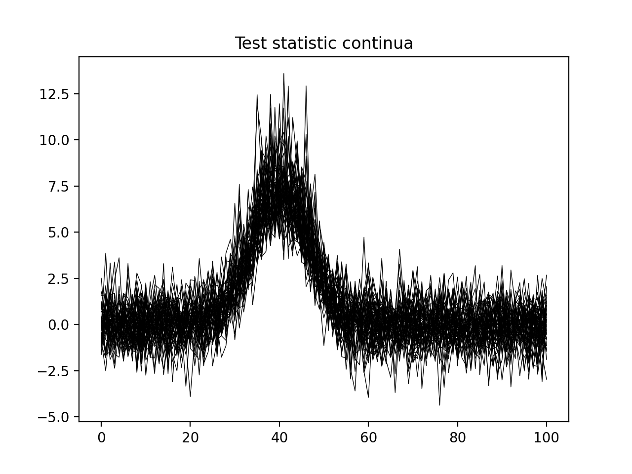
- simulate(iterations=1000, progress_bar=True)
Iteratively simulate a number of experiments.
Calling this method will repeatedly call simulate_single_iteration and will store the resulting continua in the Z attribute; if 1000 iterations are executed then Z will be a (1000,Q) array when simulation is complete.
Arguments:
iterations —- number of iterations to perform (positive int, default 1000)
progress_bar —- whether or not to display a progress bar in the terminal (bool, default True)
Example:
import numpy as np
import matplotlib.pyplot as plt
import power1d

J        = 8
Q        = 101
baseline = power1d.geom.Null( Q=Q )
signal0  = power1d.geom.Null( Q=Q )
signal1  = power1d.geom.GaussianPulse( Q=Q, q=40, fwhm=15, amp=3.5 )
noise    = power1d.noise.Gaussian( J=J, Q=Q, mu=0, sigma=1.0 )
model0   = power1d.models.DataSample(baseline, signal0, noise, J=J)
model1   = power1d.models.DataSample(baseline, signal1, noise, J=J)
emodel   = power1d.models.Experiment( [model0, model1], fn=power1d.stats.t_2sample )

emodel.simulate(iterations=50, progress_bar=True)
plt.close('all')
plt.plot( emodel.Z.T, color='k', lw=0.5 )
plt.title('Test statistic continua')
(Source code, png, hires.png, pdf)

- simulate_single_iteration()
Simulate a single experiment.
Calling this method will generate new data samples, one for each DataSample model, and will then compute and return the test statistic continuum associated with the new data samples.
ExperimentSimulator
- class power1d.models.ExperimentSimulator(model0, model1)
Two-experiment simulator.
This is a convenience class for simulating two experiments:
“null” experiment: represents the null hypothesis
“effect” experiment: represents the alternative hypothesis
Simulation results will all share the following characteristics:
Alpha-based critical thresholds are be computed for the “null” experiment
Power calculations use those thresholds to conducted power analysis on the “effect” experiment.
Arguments:
model0 —- the “null” experiment model (power1d.models.Experiment) model1 —- the “effect” experiment model (power1d.models.Experiment)
Note
If the “null” and “effect” models are identical then power will be alpha (or numerically close to it) by definition.
- Q
continuum size
- load_simulation_results(filename)
Load saved simulation results.
Arguments:
filename —- full path to saved results file
Outputs:
results —- a results object (power1d.results.SimulationResults)
Note
Simulating experiments with large sample sizes, complex DataSample models and/or a large number of simulation iterations can be computationally demanding. The load_simulation_results method allows you to probe simulation results efficiently, by saving the results to disk following simulation, then subsequently skipping the “simulate” command. In the example below the commands between the “###” flags should be commented after executing “simulate” once.
Example:
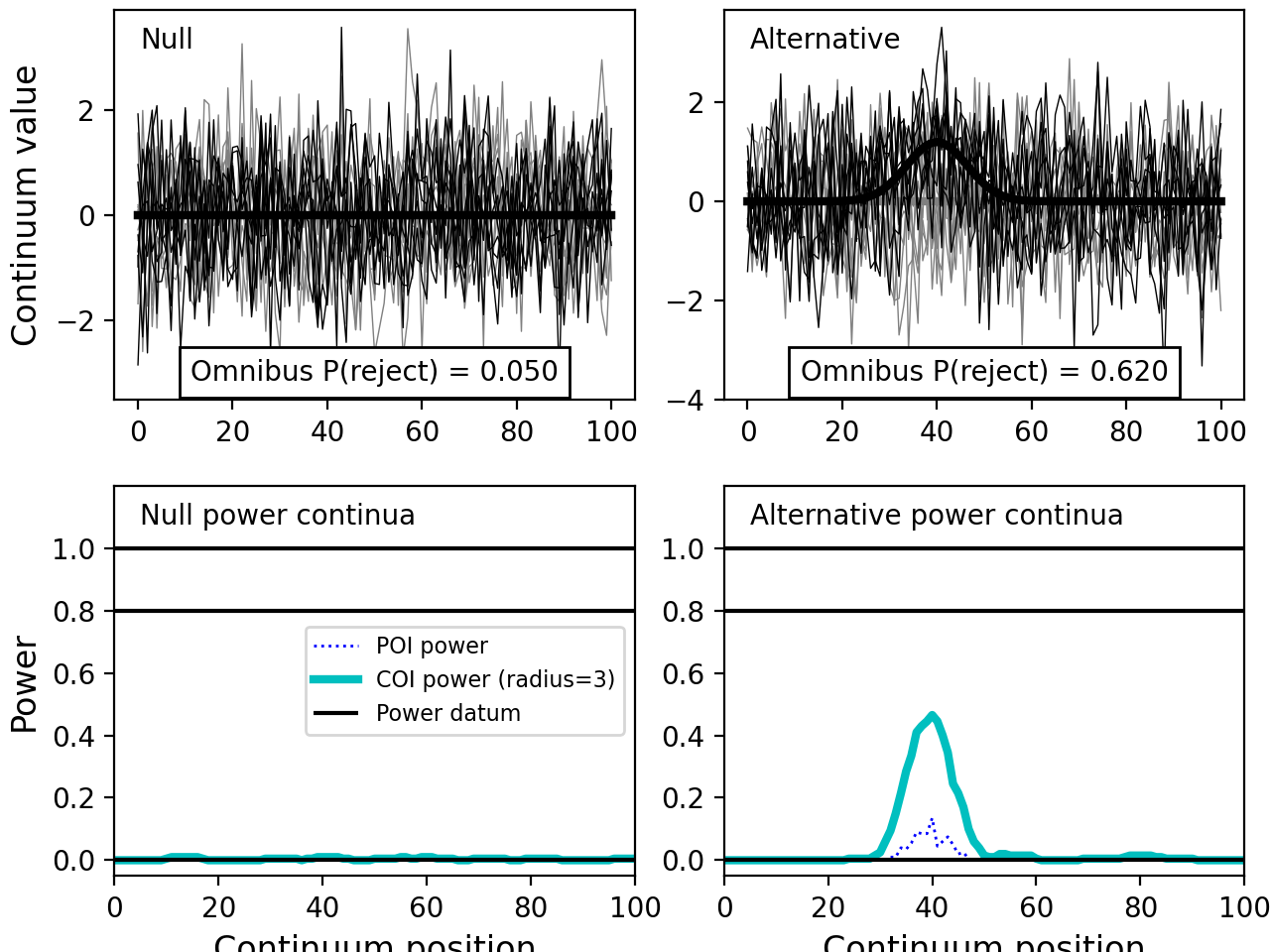
import numpy as np
import matplotlib.pyplot as plt
import power1d

J        = 8
Q        = 101
baseline = power1d.geom.Null( Q=Q )
signal0  = power1d.geom.Null( Q=Q )
signal1  = power1d.geom.GaussianPulse( Q=Q, q=40, fwhm=15, amp=1.2 )
noise    = power1d.noise.Gaussian( J=J, Q=Q, mu=0, sigma=1.0 )
model0   = power1d.models.DataSample(baseline, signal0, noise, J=J)
model1   = power1d.models.DataSample(baseline, signal1, noise, J=J)

emodel0  = power1d.models.Experiment( [model0, model0], fn=power1d.stats.t_2sample )
emodel1  = power1d.models.Experiment( [model0, model1], fn=power1d.stats.t_2sample )


###  COMMANDS BELOW SHOULD BE COMMENTED AFTER EXECUTING ONCE
sim      = power1d.models.ExperimentSimulator(emodel0, emodel1)
results  = sim.simulate(iterations=200, progress_bar=True)
fname    = "/tmp/results.npz"
results.save( fname )
###  COMMENTS ABOVE SHOULD BE COMMENTED AFTER EXECUTING ONCE

#Then the results can be re-loaded:
fname         = "/tmp/results.npz"
saved_results = sim.load_simulation_results( fname )
plt.close('all')
saved_results.plot()
(Source code, png, hires.png, pdf)

- model0
“null” experiment model
- model1
“effect” experiment model
- sample_size(power=0.8, alpha=0.05, niter0=200, niter=1000, coi=None)
Estimate sample size required to achieve a target power.
When coi is None the omnibus power is used. When coi is a dictionary then the COI power is used, e.g.
coi=dict(q=65, r=3)Arguments:
power —- target power (default: 0.8, range: [0,1])
alpha —- Type I error rate (default: 0.05, range: [0,1])
niter0 —- Number of iterations for initial, approximate solution (default: 200, range: [200,])
niter —- Number of iterations for final solution (default: 1000, range: [1000,])
coi —- Center-of-interest (default: None; either None or dict(q=q, r=r) where q is the COI and r is its radius; e.g. coi=dict(q=65, r=3))
Outputs:
Dictionary containing:
nstar —- estimated sample size required to achieve the target power
n — array of sample sizes used for the final power calculation
p — array of final power values
- simulate(iterations=50, progress_bar=True, two_tailed=False, _qprogressbar=None)
Iteratively simulate a number of experiments.
Calling this method will repeatedly call simulate_single_iteration for both the “null” model and the “effect” model.
Arguments:
iterations —- number of iterations to perform (positive int, default 1000)
progress_bar —- whether or not to display a progress bar in the terminal (bool, default True)
two_tailed —- whether or not to use two-tailed inference (bool, default False)
Outputs:
results —- a results object (power1d.results.SimulationResults)
Example:
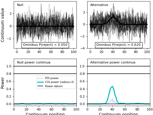
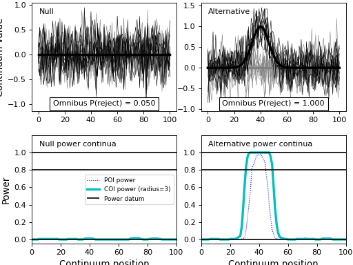
import numpy as np
import matplotlib.pyplot as plt
import power1d

J        = 8
Q        = 101
baseline = power1d.geom.Null( Q=Q )
signal0  = power1d.geom.Null( Q=Q )
signal1  = power1d.geom.GaussianPulse( Q=Q, q=40, fwhm=15, amp=1.0 )
noise    = power1d.noise.Gaussian( J=J, Q=Q, mu=0, sigma=0.3 )
model0   = power1d.models.DataSample(baseline, signal0, noise, J=J)
model1   = power1d.models.DataSample(baseline, signal1, noise, J=J)

emodel0  = power1d.models.Experiment( [model0, model0], fn=power1d.stats.t_2sample )
emodel1  = power1d.models.Experiment( [model0, model1], fn=power1d.stats.t_2sample )

sim      = power1d.models.ExperimentSimulator(emodel0, emodel1)
results  = sim.simulate(iterations=200, progress_bar=True)

plt.close('all')
results.plot()
(Source code, png, hires.png, pdf)
