Statistical testing of 1D continua
If your experimental data can be described as “1D continua” (or “1D fields” or “1D trajectories”) then Statistical Parametric Mapping (SPM) may be an appropriate statistical methodology for you to consider.
Note
SPM conducts statistical testing at the continuum level, in a conceptually simple manner. For 0D (univariate) datasets, which are the focus of most basic statistics textbooks, statistical inference stems from a model of randomness, usually the Gaussian distribution. The goal is to quantify the probability that random data would exceed a particular test statistic value (like t = 2.5 or F = 10.1). For 1D datasets, SPM-based statistical testing is conceptually identical: the goal is to quantify the probability that smooth, random 1D continua would produce a test statistic continuum whose maximum exceeds a particular test statistic value.
In spm1d statistical testing is conducted in two-stages:
Test statistic computation
Statistical inference.
This basic procedure is identical for all tests, and all test statistics.
For simplicity this document will consider just one dataset and one test.
Quick overview
The following commands execute a complete one-sample t test for a set of randomly-generated 1D continua. We shall consider these commands in more detail below.
>>> import numpy as np                 #import the numpy module (here to generate random data)
>>> from matplotlib import pyplot      #import the pyplot module (to visualize data)
>>> import spm1d                       #import the spm1d module (to conduct statistical tests and visualize 1D continua)
>>> np.random.seed(0)                  #seed the random number generator
>>> Y  = np.random.randn(10,100) +0.21  #generate 10 separate random 1D continua
>>> Y  = spm1d.util.smooth(Y, fwhm=10)  #smooth the continua
>>> t  = spm1d.stats.ttest(Y)           #conduct a one-sample t test, producing a t test statistic continuum
>>> ti = t.inference(alpha=0.05, two_tailed=False)   #conduct one-tailed inference at alpha=5%
>>> ti.plot()                          #visualize the results
>>> ti.plot_threshold_label()          #label the critical threshold
>>> ti.plot_p_values()                 #plot p values
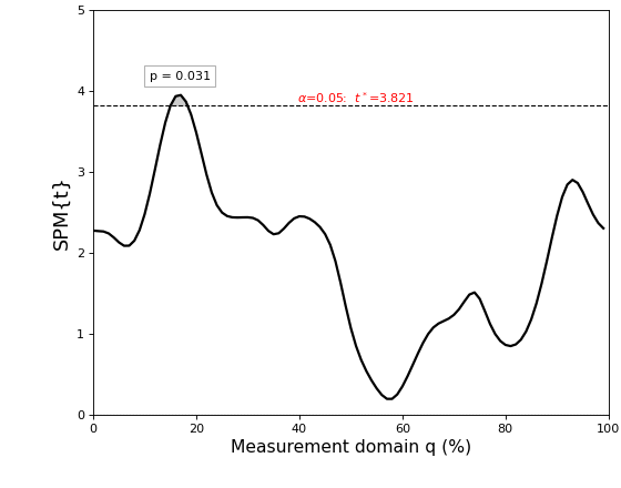
The results are depicted in the figure below.
The thick black line depicts the test statistic continuum, which in this case is a t continuum, or “SPM{t}”.
The red hashed line depicts the critical threshold at alpha = 5%. From a classical hypothesis testing perspective, the null hypothesis is rejected at alpha if the SPM{t} exceeds this threshold.
The probability (p) value indicates the probability that smooth, random continua would produce a supra-threshold cluster as broad as the observed cluster. Here “smooth” means the same smoothness as the residual continua, and “broad” means the proportion of the continuum spanned by a suprathreshold cluster.
This example is considered in extended detail below.
(Source code, png, hires.png, pdf)

Dataset
The first three lines generate smooth, random 1D continua:
>>> np.random.seed(0)
>>> Y = np.random.randn(10,100) +0.21
>>> Y = spm1d.util.smooth(Y, fwhm=10)
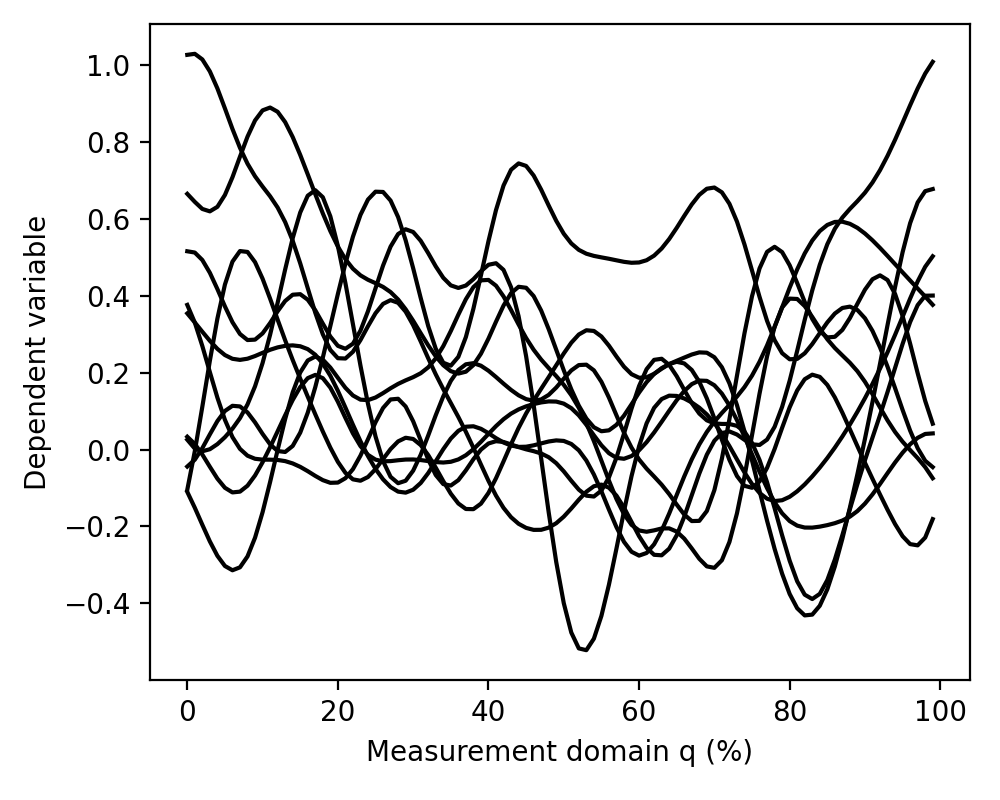
After executing these commands Y will be a (10 x 100) array containing ten separate continua, each of which has been sampled at 100 separate nodes.
The data can be visualized as follows:
>>> pyplot.plot(Y.T, color='k')
(Source code, png, hires.png, pdf)

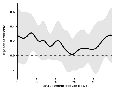
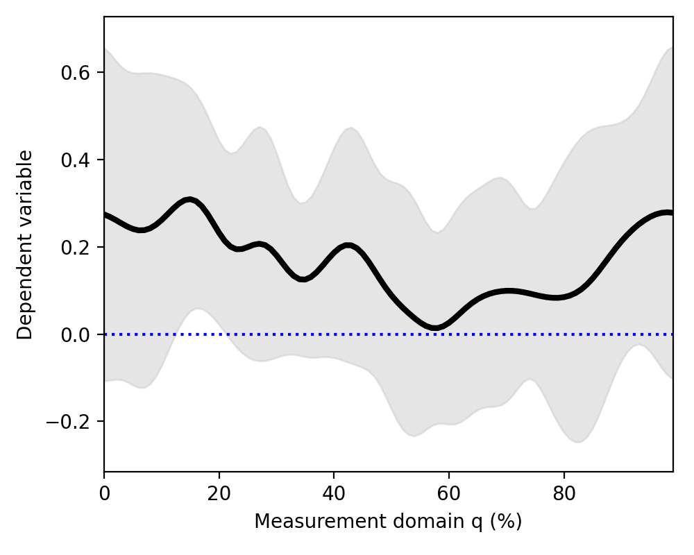
Mean continua can be visualized along with standard deviation (SD) clouds like this:
>>> spm1d.plot.plot_mean_sd(Y)
>>> pyplot.plot([0,100], [0,0], 'b:')
(Source code, png, hires.png, pdf)

Warning
Although the mean minus SD exceeds zero in the vicinity of q = 18%, implying that this is the strongest signal, this observation has no probabilistic meaning.
For objective reporting we need to quantify the probability that random data would produce a signal as large or larger than this signal, given the variability.
However, before computing that probability we need to compute a test statistic, which has known probabilistic behavior in an infinite number of experiments.
Test statistic computation
In spm1d you can compute the test statistic for the one-sample t test as follows:
>>> t = spm1d.stats.ttest(Y)
The result t is a 1D test statistic continuum, or equivalently a “Statistical Parametric Map” (SPM), denoted “SPM{t}”. It can be visualized as follows:
>>> t.plot()
(Source code, png, hires.png, pdf)
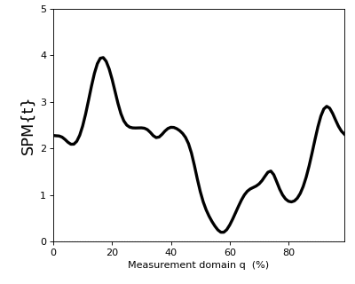
In addition to visualizing the results, as in the figure above, you can also probe SPM attributes as described in Test outputs.
Danger
Do not misinterpret test statistic estimation at 100 nodes as equivalent to having conducted 100 separate statistical tests. Such an interpretation would be incorrect on two counts. First, estimating the test statistic at multiple nodes, just like estimating the mean at multiple nodes, results in just one continuum estimate. Thus the number of nodes is irrelevant; there will always be just one test statistic continuum. Second, computing the test statistic does not constitute statistical testing. Indeed, at this point we have conducted precisely zero statistical tests. A statistical test is conducted only when we quantify the probability that random data would produce particular features of our test statistic. If the test statistic is a 0D scalar (e.g. t = 3.1), then the goal is to quantify the probability that random data would produce a t value as large or larger than the observed value. If the test statistic is a 1D continuum, then the goal is to quantify the probability that random continua would produce particular geometric features in test statistic continua, like maximum continuum height.
Statistical inference
In spm1d statistical inference is conducted separately from test statistic computation as follows:
>>> t  = spm1d.stats.ttest(Y)
>>> ti = t.inference(alpha=0.05, two_tailed=False)
Warning
By default spm1d conducts two-tailed inference. To force one-tailed inference set the keyword two_tailed to False, as indicated above. A discussion of one- vs. two-tailed inference can be found here: One- vs. two-tailed inference.
Note
We have set an a priori Type I error rate of alpha = 5%. If the data are 0D scalars, and if we have conducted a t test, then alpha maps directly to a single critical t value, which we shall denote t*. If the observed t value exceeds t*, then from a classical hypothesis testing perspective the test is said to be significant at a Type I error rate of alpha. Similarly, alpha also maps to a generally different threshold t* when the data are 1D continua. In the 1D case, alpha pertains to the maximum t value across the entire continuum, and ensures that random continua reach t* with a probability of alpha.
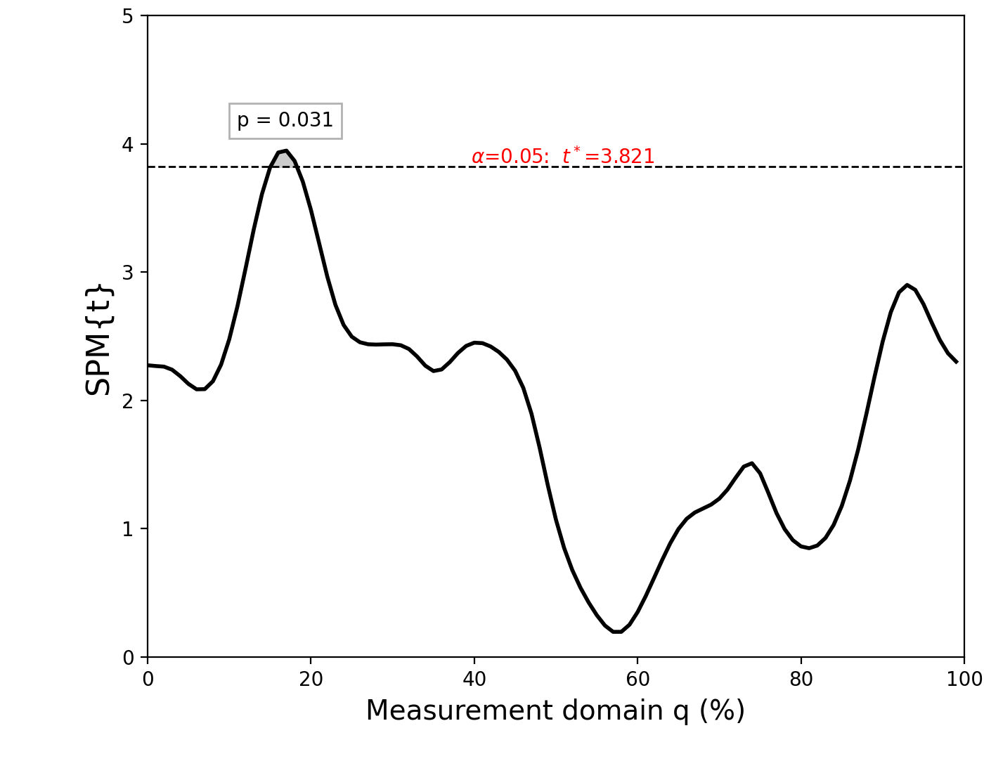
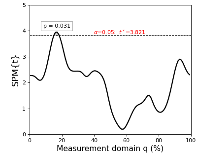
The inference SPM{t} can be visualized using:
>>> ti.plot()
>>> ti.plot_threshold_label(fontsize=10)
>>> ti.plot_p_values(size=10, offsets=[(0,0.3)])
The size keyword argument specifies the font size for the p value text, and the offsets keyword argument specifies where to position the text relative to the cluster centroid.
Alternatively you can plot p values manually using pyplot.text, like this:
>>> pyplot.text(5, 4.1, 'p = %.3f' %ti.p[0], size=10)
You can also probe inference results interactively as described in Inference SPMs.
The resulting figure (below) depicts the raw SPM{t} along with the alpha-based critical threshold t* and the probability value associated with the suprathreshold cluster.
(Source code, png, hires.png, pdf)
Note
The probability that smooth random continua will produce an SPM{t} that reaches t* is precisely alpha. If the test statistic continuum just touches the critical threshold, then by definition the p value is alpha. As the test statistic continuum traverses beyond the critical threshold, as in the example above, the p value gets progressively smaller. The p value specifies the probability that smooth random fields would produce a suprathreshold cluster as broad or broader than the observed cluster, where “broad” refers to the width of the cluster relative to the width of the whole continuum.
Danger
Do not misinterpret alpha, t* or p values as descriptive elements of a particular dataset. Instead they describe random data behavior.