Basic

Generating 1D Gaussian fields

Smooth 1D Gaussian fields can be generated using the rft1d.randn1d function:

>>> import rft1d
>>> nResponses = 5
>>> nNodes = 101
>>> FWHM = 10.0
>>> y = rft1d.randn1d(nResponses, nNodes, FWHM)

The generated fields are stored in a 2D NumPy array with shape = (nResponses, nNodes). They can thus be visualized easily using matplotlib:

>>> from matplotlib import pyplot
>>> pyplot.plot(y.T)

(Source code, png, hires.png, pdf)

If simulating random fields over many iterations the rft1d.Generator1D is slightly faster:

>>> g = rft1d.Generator1D(nResponses=8, nNodes=101, FWHM=10.0)
>>> yA = g.generate_array()
>>> yB = g.generate_array()
>>> yC = g.generate_array()

Warning

Generating very smooth random fields requires field padding to adhere to RFT expectations. This can be done easily using the pad keyword argument, but this becomes increasingly slow as FWHM increases.

>>> y = rft1d.randn1d(5, 101, 80.0, pad=True)
>>> g = rft1d.Generator1D(5, 101, 80.0, pad=True)
>>> y = g.generate_array()

Increasing the FWHM in this manner yields much smoother fields; below is an example of FWHM=80.0.

(Source code, png, hires.png, pdf)

Reproducing 1D Gaussian fields

To precisely reproduce partcular random fields, use np.random.seed:

>>> import numpy as np
>>> import rft1d
>>> np.random.seed(0)
>>> a = rft1d.randn1d(5, 101, 20.0)
>>> b = rft1d.randn1d(5, 101, 20.0)  # a and b are different
>>> np.random.seed(0)
>>> c = rft1d.randn1d(5, 101, 20.0)  # a and c are identical

Node-based vs. element-based sampling

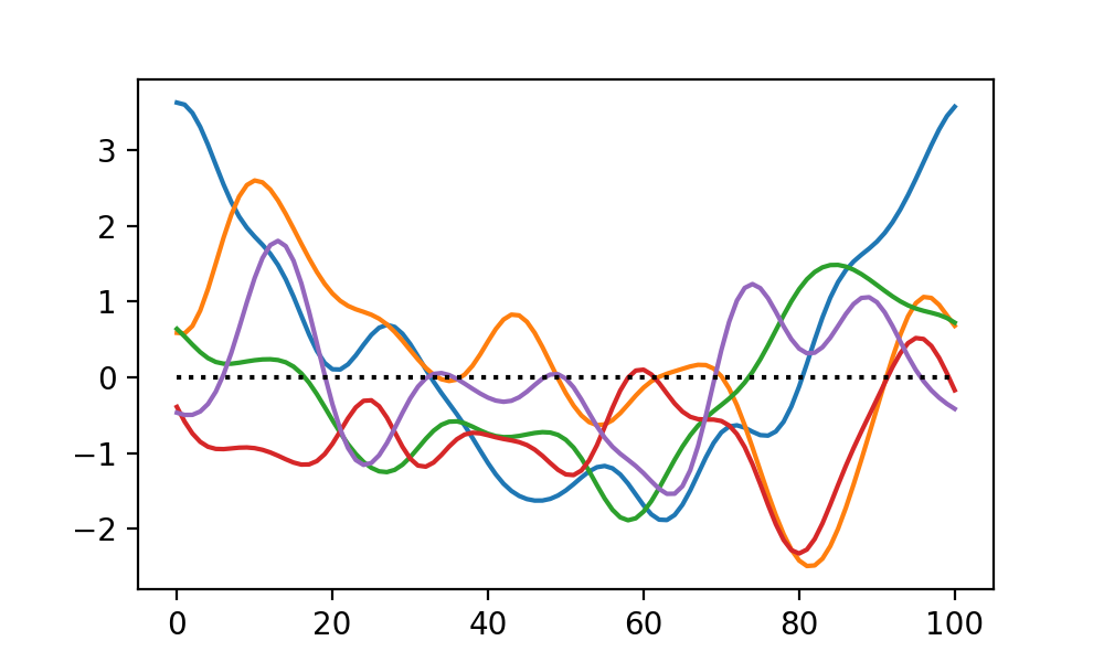
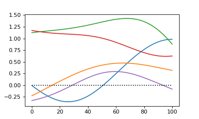
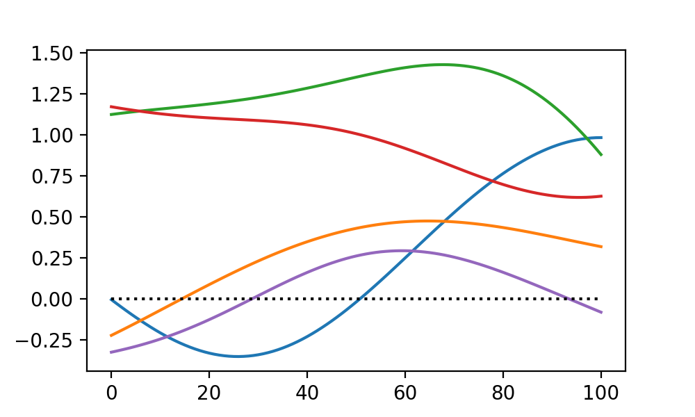
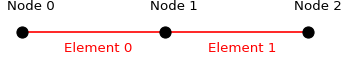
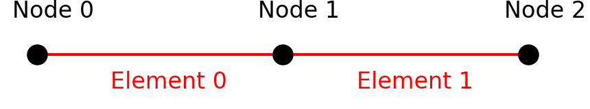
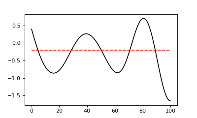
Fields may be sampled either in a node-based sense or in an element-based sense. As suggested by the figure below, node-based sampling refers to discrete measurements at single instants in time or at single points in space. Element-based sampling, on the other hand, refers to measurements that span an interval.

(Source code, png, hires.png, pdf)

Some common examples of each:

Node-based sampling:

• Biomechanical time series (sampled at discrete instants)

• Ocean wave heights (sampled by discrete sensors)

Element-based sampling:

• Contact pressure distribution (average pressure acting over an area)

• Long-interval time series (sampled daily, weekly or monthly, where each sample represents one whole day, week or month)

Node-based sampling is assumed by default in rft1d. Switching to element-based sampling can be done by setting the keyword “element_based” to True in relevant rft1d procedures.

Extracting maxima

Since the fields are NumPy arrays field maxima can be extracted using np.max and np.argmax:

>>> y = rft1d.randn1d(5, 101, 25.0)
>>> ymax = y.max(axis=1)
>>> x = y.argmax(axis=1)
>>> pyplot.plot(y.T, 'k')
>>> pyplot.plot(x, ymax, 'ro')

(Source code, png, hires.png, pdf)

Computing upcrossing metrics

Consider the following random field thresholded at a height of -0.2, for which there are three upcrossings.

(Source code, png, hires.png, pdf)

Let’s zoom in on the first upcrossing to give a clearer context to upcrossing metric results below.

(Source code, png, hires.png, pdf)

To compute upcrossing metrics set a height u then use the rft1d.geom.ClusterMetricCalculator class.

>>>  np.random.seed(3)
>>>  y = rft1d.randn1d(1, 101, 20.0, pad=True)
>>>  calc = rft1d.geom.ClusterMetricCalculator()
>>>  u = -0.2
>>>  print calc.cluster_extents(y, u) #yields [3.54, 21.3, 18.2]
>>>  print calc.max_cluster_extent(y, u) #yields 21.3
>>>  print calc.mean_cluster_extent(y, u) #yields 14.4
>>>  print calc.nSuprathresholdNodes(y, u) #yields 45
>>>  print calc.nSuprathresholdResels(y, u, fwhm=10) #yields 4.31
>>>  print calc.nUpcrossings(y, u) #yields 3
>>>  print calc.nUpcrossingsByExtent(y, u, 5) #yields 2

Note

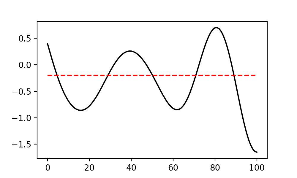
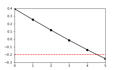
There are four supra-threshold nodes in the first upcrossing shown above, but the length of the upcrossing (i.e. its extent) is less than four. From the procedures above, cluster_extents and nSuprathresholdResels are reported as lengths.

By default cluster extents are interpolated to the threshold u. Disabling interpolation using the keyword interp is faster, and will yield integer extents:

>>>  print calc.cluster_extents(y, u, interp=False) #yields [3, 21, 18]
>>>  print calc.max_cluster_extent(y, u, interp=False) #yields 21
>>>  print calc.mean_cluster_extent(y, u, interp=False) #yields 14

Danger

Setting interp to False is faster, but it may cause disagreements between node-based and element-based sampling (if only one node exceeds u, the node-based extent is zero, but the element-based extent may be zero or one). If the upcrossing is large this difference is negligible, but for small upcrossing there may be strange results (i.e. upcrossing with an extent of zero). Recommendation: always interpolate.

Checking RFT expectations

RFT expectations regarding Gaussian random fields can be accessed via an interface similar to scipy.stats. As an example, in scipy the survival function for the standard normal distribution is given by:

>>>  from scipy import stats
>>>  stats.norm.sf(2.0) #yields 0.023

In rft1d the survival function for standard normal Gaussian fields is given by:

>>>  nNodes = 101
>>>  FWHM = 10.0
>>>  print rft1d.norm.sf(2.0, nNodes, FWHM) #yields 0.320

Thus a 1D Gaussian random field with FWHM=10 and a field length of 100 is about 14 times more likely to reach a height of 2.0 than is a 0D Gaussian scalar.

The most convenient way to explore RFT expectations and probabilities is with the rft1d.prob.RFTCalculator class:

>>> calc = rft1d.prob.RFTCalculator('T', (1,8), 101, 15.0)
>>> print calc.expected.number_of_upcrossings(1.0) #yields 1.343
>>> print calc.expected.number_of_upcrossings(4.5) #yields 0.0223
>>> print calc.expected.nodes_per_upcrossing(2.0)  #yields 10.419
>>> print calc.p.upcrossing(3.0)  #yields 0.126

Note

The minum value of expected.nodes_per_upcrossing is one because, if there is an upcrossing, it must have at least one node.

Validating RFT expectations

RFT expectations can be validated as follows:

1. Use rft1d.prob.RFTCalculator to generate theoretical predictions (see here)

2. Then use rft1d.randn1d to generate random fields (see here)

3. For each random field use rft1d.geom.ClusterMetricCalculator to compute upcrossing metrics (see here)

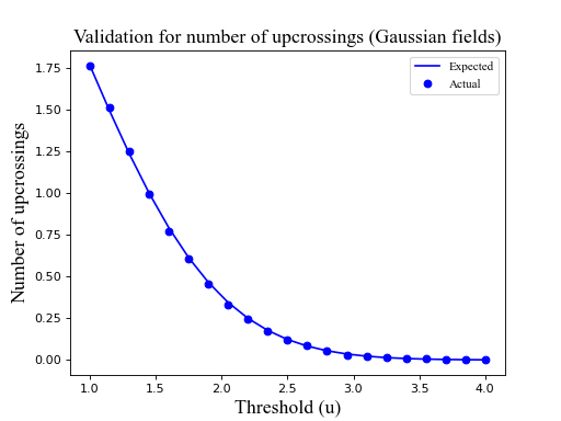
The figure below depicts a validation for the expected number of upcrossings in Gaussian fields with FWHM=10. Click on the “source code” link below to see details.

(Source code, png, hires.png, pdf)