power1d.noise¶

One-dimensional noise models.

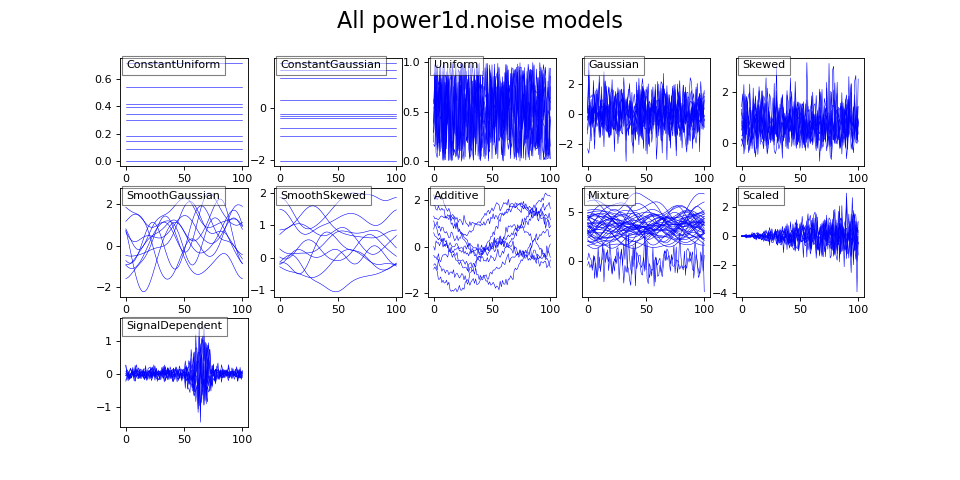
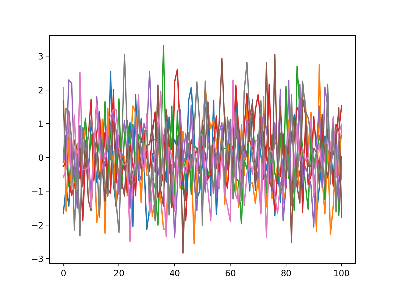
The figure below provides overview of all noise types. Details regarding reach are listed below.

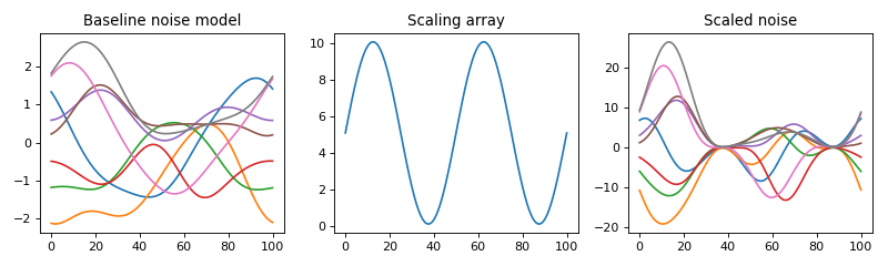
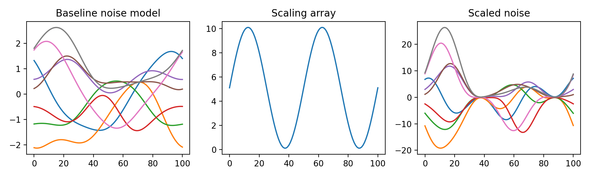
from_array¶

power1d.noise.from_array(noise, x)¶

Create Scaled noise object from a 1D array.

This function is equivalent to creating a Scaled noise object.

While redundant this function is included for API consistency, as a sister-function to geom.from_array and models.datasample_from_array

Arguments:

noise —- a Noise object

x —- scaling array (1D numpy array)

Outputs:

obj —- a Scaled noise object

Example:

import numpy as np
import matplotlib.pyplot as plt
import power1d

J      = 8  # sample size
Q      = 101  # number of continuum nodes
x      = 5.1 + 5 * np.sin( np.linspace(0, 4*np.pi, Q) )
noise  = power1d.noise.SmoothGaussian( J, Q, fwhm=30 ) # baseline noise model
snoise = power1d.noise.from_array( noise, x ) # scaled noise object

fig,axs = plt.subplots(1, 3, figsize=(10,3), tight_layout=True)
noise.plot( ax=axs[0] )
axs[1].plot( x )
snoise.plot( ax=axs[2] )
labels  = 'Baseline noise model', 'Scaling array', 'Scaled noise'
[ax.set_title(s) for ax,s in zip(axs,labels)]
plt.show()

(Source code, png, hires.png, pdf)

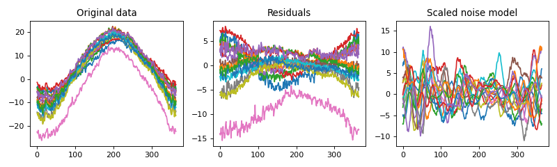
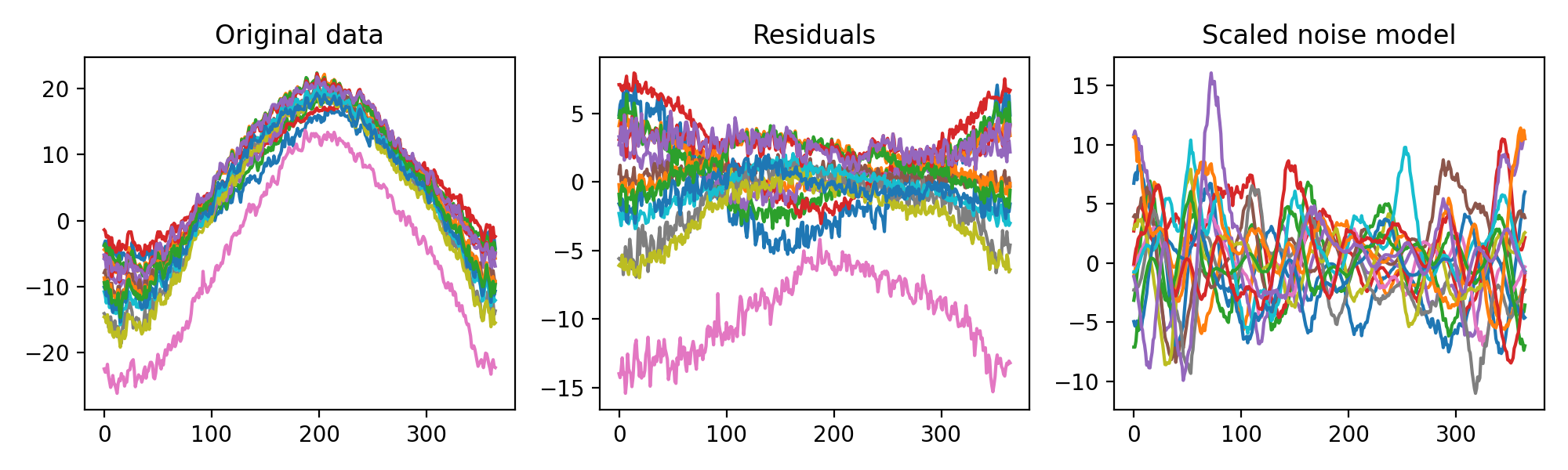
from_residuals¶

power1d.noise.from_residuals(r, pad=False)¶

Convenience function for creating Scaled noise objects from sets of experimental residuals.

The mean of the residuals must be zero (i.e., the null continuum)

WARNING! As shown in the example below, “from_residuals” may produce a noise model that does NOT embody all features of the residuals. In this case more complex noise modeling (e.g. Additive, Mixture) may be required.

Arguments:

r —- a (J,Q) array of experimental residuals (J=observations, Q=domain nodes)

Outputs:

obj —- a Scaled noise object

Example:

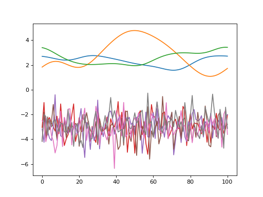
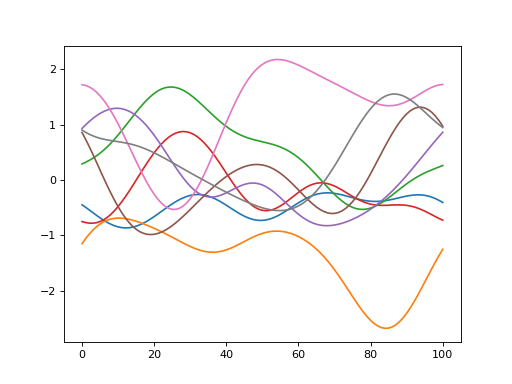
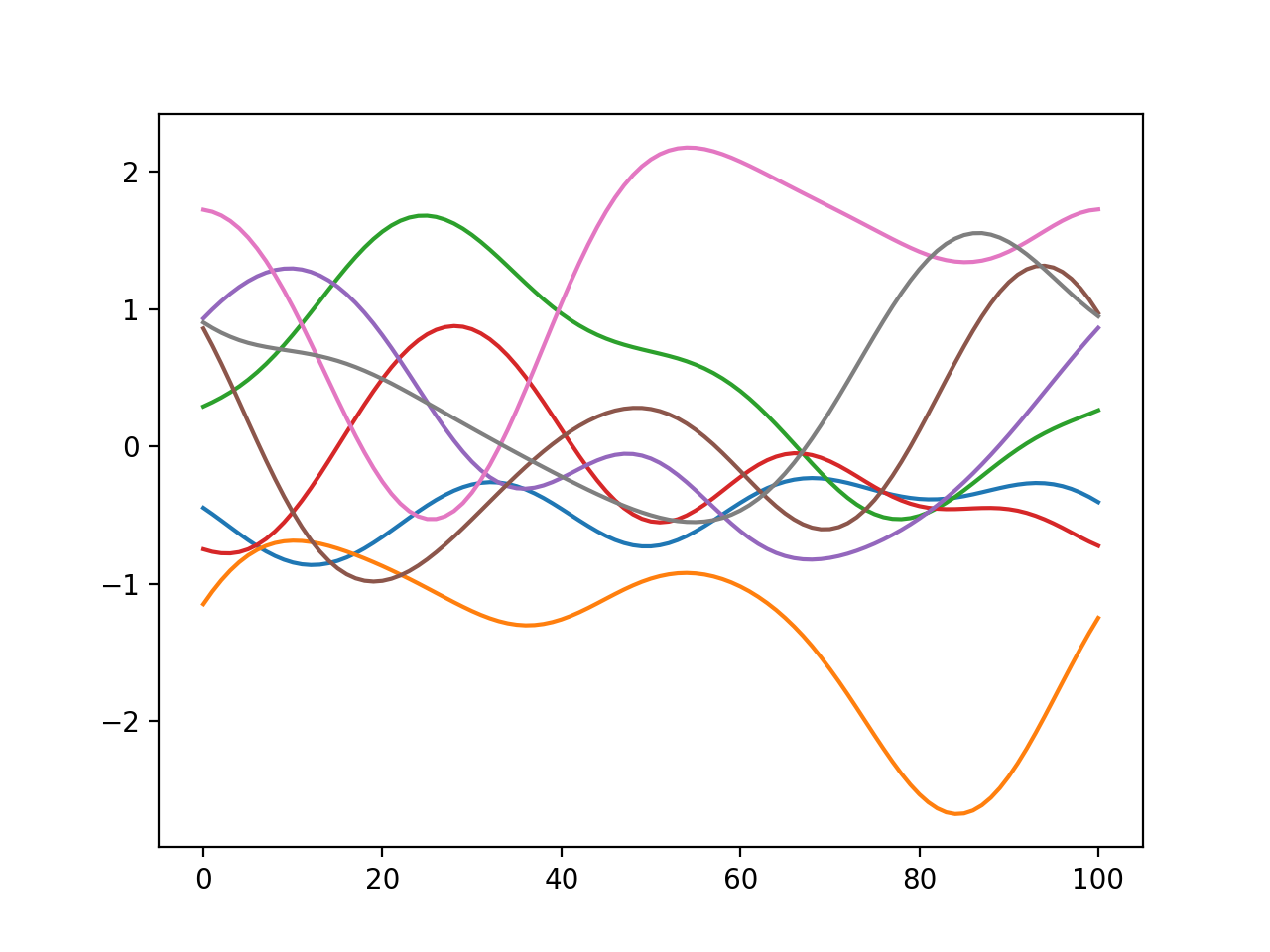
import numpy as np
import matplotlib.pyplot as plt
import power1d

y      = power1d.data.weather()['Atlantic']
r      = y - y.mean( axis=0 ) # residuals
snoise = power1d.noise.from_residuals( r ) # scaled noise object

fig,axs = plt.subplots(1, 3, figsize=(10,3), tight_layout=True)
axs[0].plot( y.T )
axs[1].plot( r.T )
snoise.plot( ax=axs[2] )
labels  = 'Original data', 'Residuals', 'Scaled noise model'
[ax.set_title(s) for ax,s in zip(axs,labels)]
plt.show()

(Source code, png, hires.png, pdf)

Additive¶

power1d.noise.Additive(*noise_models)¶

Additive model (sum of two or more other noise types.)

Arguments:

A sequence of power1d.noise models (must have the same shape: (J,Q) )

Example:

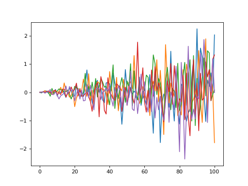
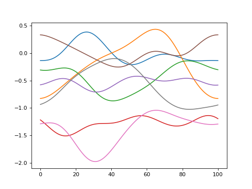
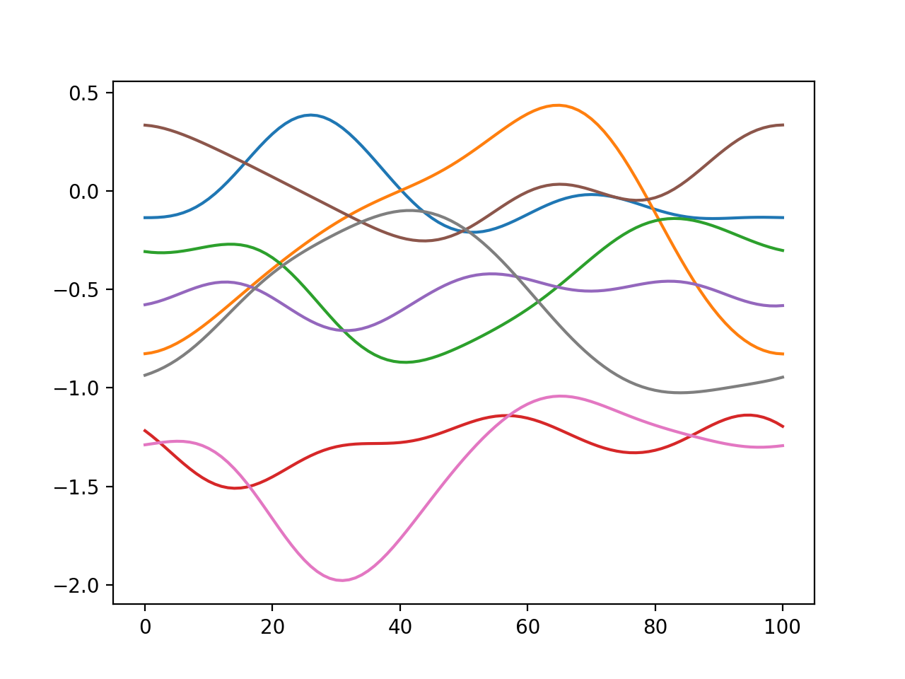
import power1d

noise0  = power1d.noise.SmoothGaussian( J=8, Q=501, mu=0, sigma=1.0, fwhm=100 )
noise1  = power1d.noise.Gaussian( J=8, Q=501, mu=0, sigma=0.1 )
noise   = power1d.noise.Additive(noise0, noise1)
noise.plot()

(Source code, png, hires.png, pdf)

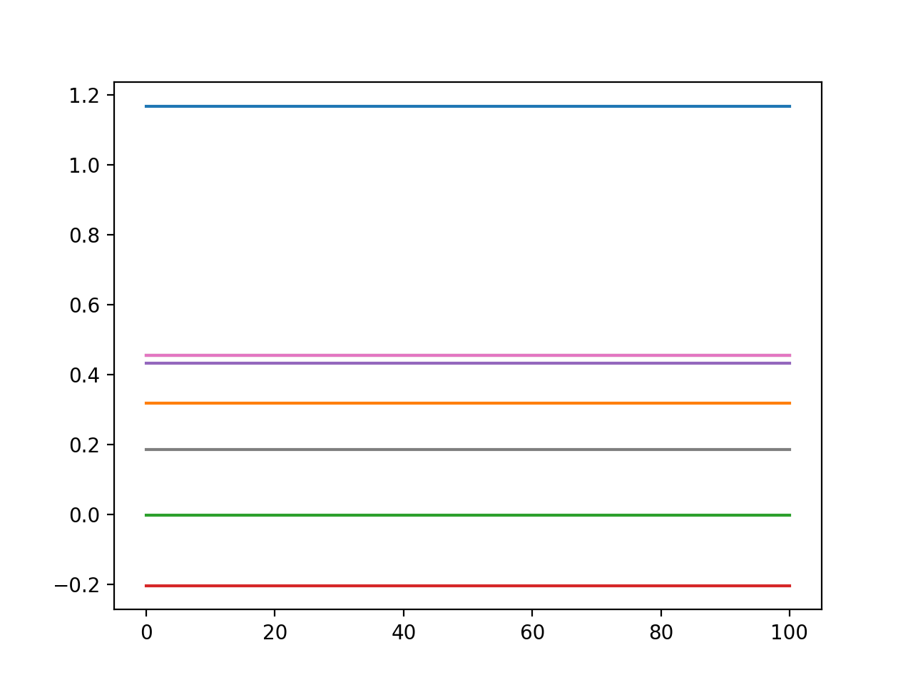
ConstantGaussian¶

power1d.noise.ConstantGaussian(J=1, Q=101, mu=0, sigma=1)¶

Gaussian-distributed constant continuum noise.

Each of the J continua has a constant value, and these values are distributed normally according to mu and sigma.

Arguments:

J —- sample size (int) (default 1)

Q —- continuum size (int) (default 101)

x0 —- minimum value (float or int) (default 0)

x1 —- maximum value (float or int) (default 1)

Example:

import power1d

noise   = power1d.noise.ConstantGaussian( J=8, Q=101, mu=0, sigma=1.0 )
noise.plot()

(Source code, png, hires.png, pdf)

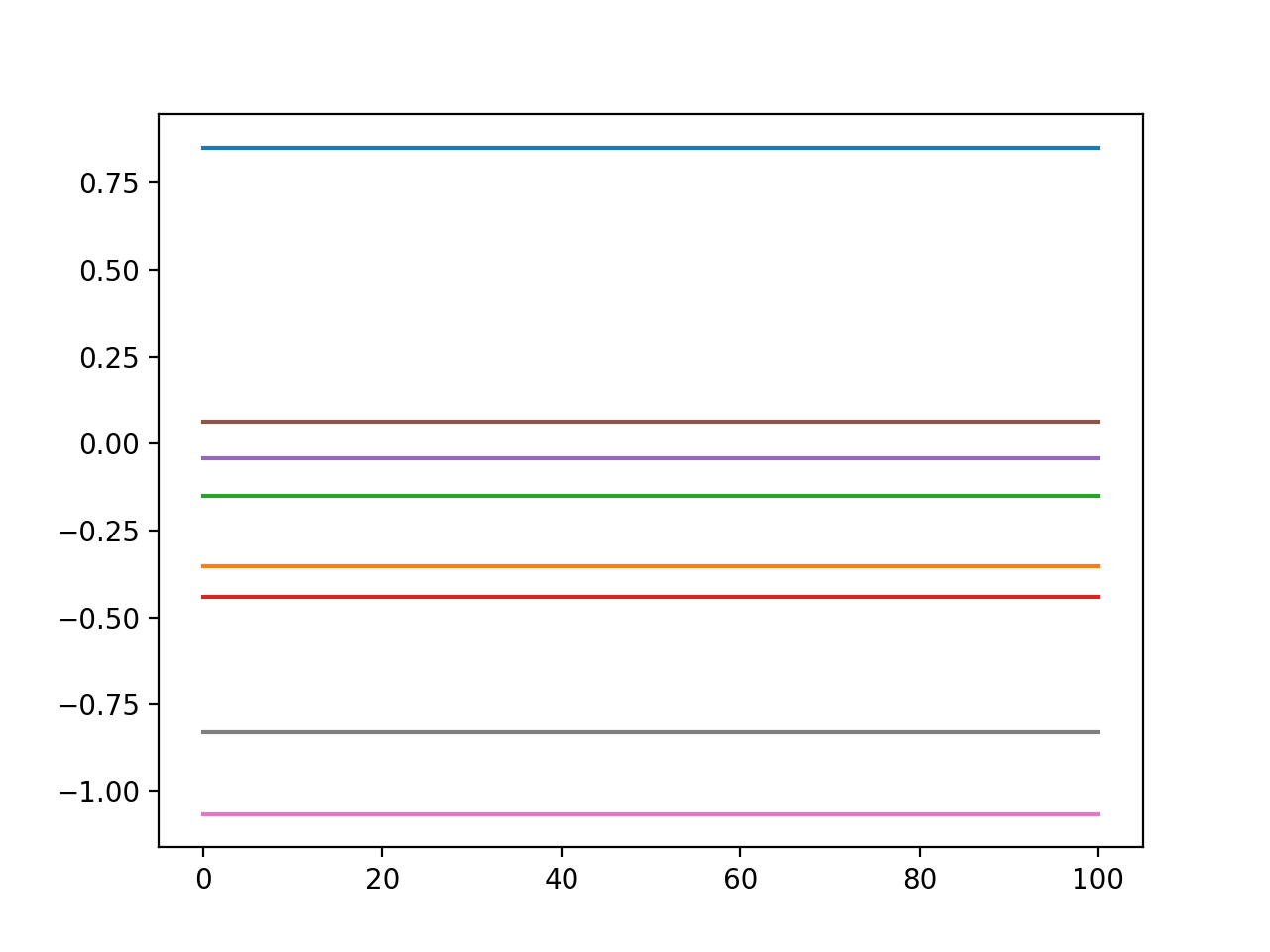
ConstantUniform¶

power1d.noise.ConstantUniform(J=1, Q=101, x0=0, x1=1)¶

Uniformly-distributed constant continuum noise.

Each of the J continua has a constant value, and these values are distributed uniformly between x0 and x1.

Arguments:

J —- sample size (int) (default 1)

Q —- continuum size (int) (default 101)

x0 —- mean (float or int) (default 0)

x1 —- standard deviation (float or int) (default 1)

Example:

import power1d

noise   = power1d.noise.ConstantUniform( J=8, Q=101, x0=-0.5, x1=1.3 )
noise.plot()

(Source code, png, hires.png, pdf)

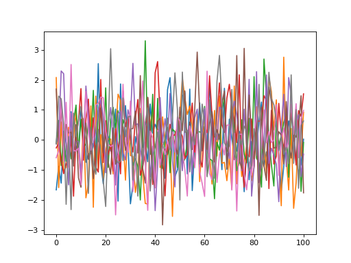
Gaussian¶

power1d.noise.Gaussian(J=1, Q=101, mu=0, sigma=1)¶

Uncorrelated Gaussian noise.

Arguments:

J —- sample size (int) (default 1)

Q —- continuum size (int) (default 101)

mu —- mean (float or int) (default 0)

sigma —- standard deviation (float or int) (default 1)

Example:

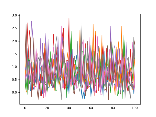
import power1d

noise   = power1d.noise.Gaussian( J=8, Q=101, mu=0, sigma=1.0 )
noise.plot()

(Source code, png, hires.png, pdf)

Mixture¶

power1d.noise.Mixture(*noise_models)¶

Noise mixture model (mixture of noise types in a fixed ratio)

Arguments:

A sequence of power1d.noise models (must have the same shape: (,Q) )

Example:

import power1d

noise0  = power1d.noise.SmoothGaussian( J=3, Q=101, mu=3, sigma=1.0, fwhm=20 )
noise1  = power1d.noise.Gaussian( J=5, Q=101, mu=-3, sigma=1.0 )
noise   = power1d.noise.Mixture(noise0, noise1)
noise.plot()

(Source code, png, hires.png, pdf)

Scaled¶

power1d.noise.Scaled(noise, scale)¶

Scaled noise model.

Arguments:

noise —- a power1d.noise object

scale —- a numpy array or a power1d.primitive object

Example:

import numpy as np
import power1d

Q       = 101
noise0  = power1d.noise.Gaussian( J=5, Q=Q, mu=0, sigma=1.0 )
scale   = np.linspace(0, 1, Q)
noise   = power1d.noise.Scaled(noise0, scale)
noise.plot()

(Source code, png, hires.png, pdf)

SignalDependent¶

power1d.noise.SignalDependent(noise, signal, fn=None)¶

Signal-dependent noise model.

Arguments:

noise —- a power1d.noise object

signal —- a numpy array or a power1d.signal object

fn —- an arbitrary function of noise and signal (default fn = lambda n,s: n + (n * s))

Example:

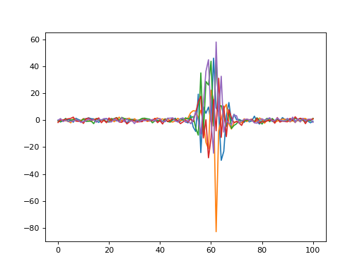
import numpy as np
import power1d

Q       = 101
noise0  = power1d.noise.Gaussian( J=5, Q=Q, mu=0, sigma=1.0 )
signal  = power1d.geom.GaussianPulse(Q=Q, q=60, amp=3, fwhm=15)
fn      = lambda n,s: n + (n * s**3)
noise   = power1d.noise.SignalDependent(noise0, signal, fn)
noise.plot()

(Source code, png, hires.png, pdf)

power1d.noise.Skewed(J=8, Q=101, mu=0, sigma=1, alpha=0)¶

Skewed noise.

Warning

Skewed distributions are approximate and may not be consistent with theoretical solutions. In particular the their maximum likelihoods are not mu. In power1d skewed distribution are meant only to be used as tools to approximate experimentally observed skewed noise and / or for exploratory purposes (i.e. to examine power changes associated with roughly skewed distributions).

Arguments:

J —- sample size (int) (default 1)

Q —- continuum size (int) (default 101)

mu —- mean (float or int) (default 0)

sigma —- standard deviation (float or int) (default 1)

alpha —- skewness (float or int) (default 0)

Modified from a StackOverflow contribution by jamesj629:

http://stackoverflow.com/questions/36200913/generate-n-random-numbers-from-a-skew-normal-distribution-using-numpy

Example:

import power1d

noise   = power1d.noise.Skewed( J=8, Q=101, mu=0, sigma=1.0, alpha=5 )
noise.plot()

(Source code, png, hires.png, pdf)

SmoothGaussian¶

power1d.noise.SmoothGaussian(J=1, Q=101, mu=0, sigma=1, fwhm=20, pad=False)¶

Smooth (correlated) Gaussian noise.

Arguments:

J —- sample size (int) (default 1)

Q —- continuum size (int) (default 101)

mu —- mean (float or int) (default 0)

sigma —- standard deviation (float or int) (default 1)

fwhm —- smoothness (float or int) (default 20); this is the full-width-at-half-maximum of a Gaussian kernel which is convolved with uncorrelated Gaussian noise; the resulting smooth noise is re-scaled to unit variance

pad —- whether to pad continuum when smoothing (True or False) (default False); unpadded noise has the same value at the beginning and end of the continuum

Example:

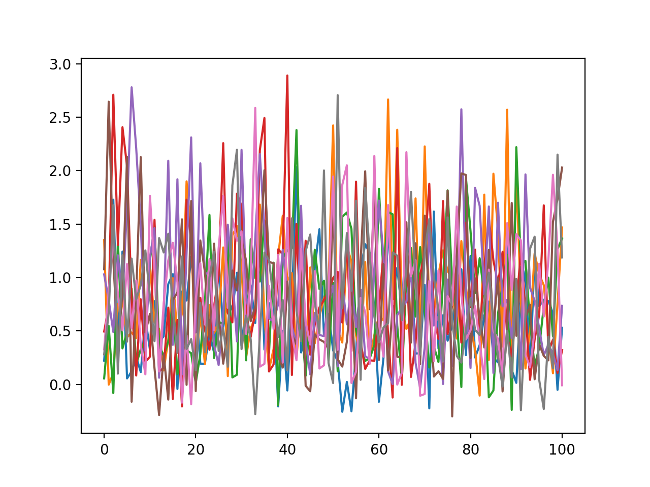
import power1d

noise   = power1d.noise.SmoothGaussian( J=8, Q=101, mu=0, sigma=1.0, fwhm=25, pad=False )
noise.plot()

(Source code, png, hires.png, pdf)

SmoothSkewed¶

power1d.noise.SmoothSkewed(J=8, Q=101, mu=0, sigma=1, fwhm=20, pad=True, alpha=0)¶

Smooth, skewed noise.

Warning

This smooth skewed distribution implementation is preliminary and will only accept skewness parameter “alpha” values in the range (1, 5). To skew in the opposite direction use (-5, -1). Note that skewed distributions are approximate and may not be consistent with theoretical solutions.

Arguments:

J —- sample size (int) (default 1)

Q —- continuum size (int) (default 101)

mu —- mean (float or int) (default 0)

sigma —- standard deviation (float or int) (default 1)

fwhm —- smoothness (float or int) (default 20); this is the full-width-at-half-maximum of a Gaussian kernel which is convolved with uncorrelated Gaussian noise; the resulting smooth noise is re-scaled to unit variance

pad —- whether to pad continuum when smoothing (True or False) (default False); unpadded noise has the same value at the beginning and end of the continuum

alpha —- skewness (float or int between -5 and 5) (default 0)

Example:

import power1d

noise   = power1d.noise.SmoothSkewed( J=8, Q=101, mu=0, sigma=1.0, fwhm=25, pad=False, alpha=-3 )
noise.plot()

(Source code, png, hires.png, pdf)

Uniform¶

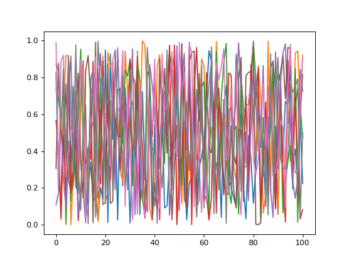
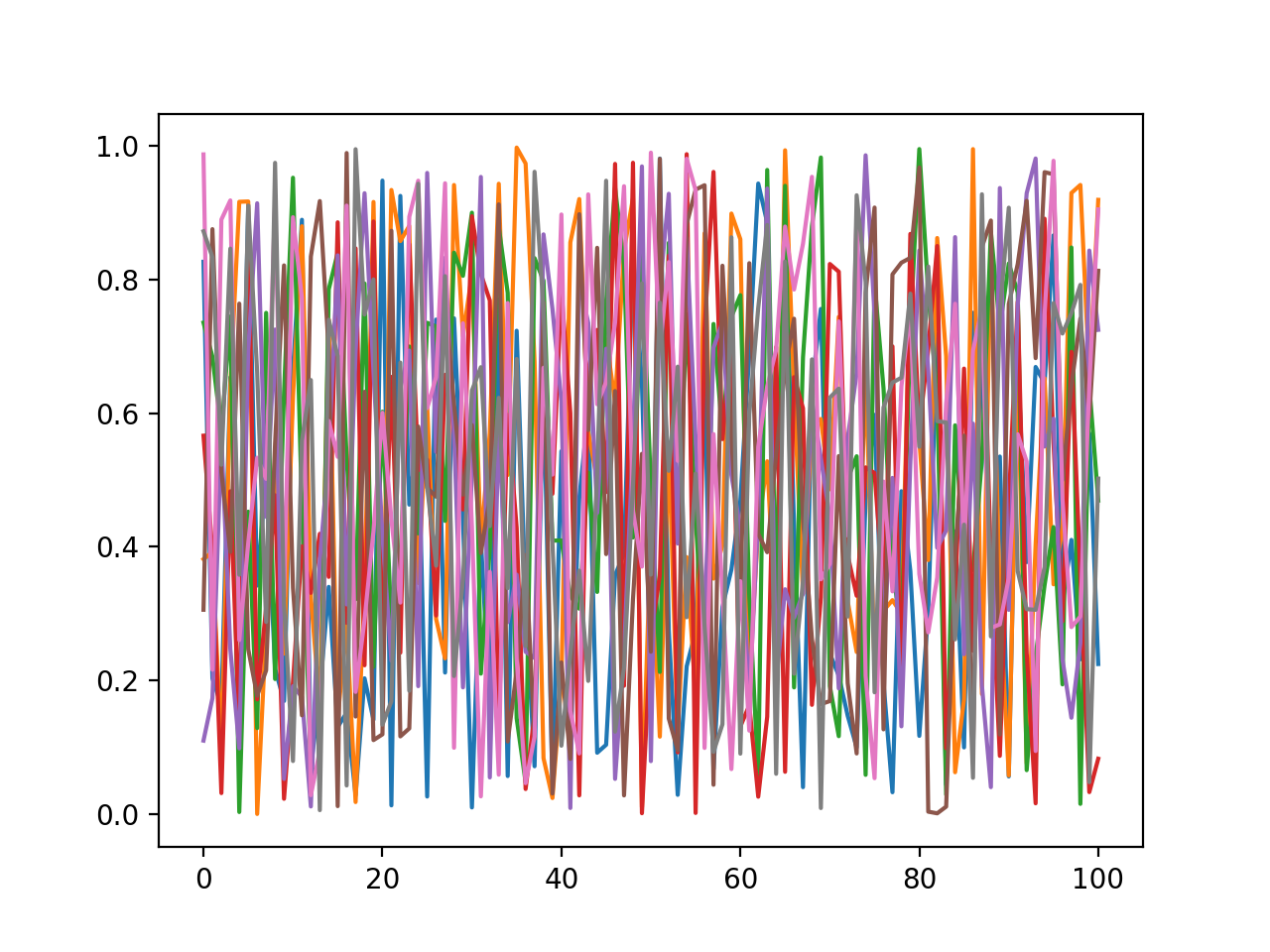
power1d.noise.Uniform(J=1, Q=101, x0=0, x1=1)¶

Uniform noise.

Arguments:

J —- sample size (int) (default 1)

Q —- continuum size (int) (default 101)

x0 —- minimum value (float or int) (default 0)

x1 —- maximum value (float or int) (default 1)

Example:

import power1d

noise   = power1d.noise.Uniform( J=8, Q=101, x0=0, x1=1.0 )
noise.plot()

(Source code, png, hires.png, pdf)

power1d.noise¶

from_array¶

from_residuals¶

Additive¶

ConstantGaussian¶

ConstantUniform¶

Gaussian¶

Mixture¶

Scaled¶

SignalDependent¶

SmoothGaussian¶

SmoothSkewed¶

Uniform¶

Table of Contents

Previous topic

Next topic

This Page