power1d.results
A module for probing, displaying and plotting power1d simulation results.
This module contains the SimulationResults class which is meant to be instantiated only by power1d and not by the user. However, once instantiated the user can run a variety of analyses using the methods described below.
Importantly, since simualations can take a long time to run users are encouraged to save SimulationResults objects using the “save” method and re-loaded using the load_simulation_results method of an ExperimentSimulator object.
Example:
import numpy as np
import matplotlib.pyplot as plt
import power1d
J = 8
Q = 101
baseline = power1d.geom.Null( Q=Q )
signal0 = power1d.geom.Null( Q=Q )
signal1 = power1d.geom.GaussianPulse( Q=Q, q=40, fwhm=15, amp=1.0 )
noise = power1d.noise.Gaussian( J=J, Q=Q, mu=0, sigma=0.3 )
model0 = power1d.models.DataSample(baseline, signal0, noise, J=J)
model1 = power1d.models.DataSample(baseline, signal1, noise, J=J)
emodel0 = power1d.models.Experiment( [model0, model0], fn=power1d.stats.t_2sample )
emodel1 = power1d.models.Experiment( [model0, model1], fn=power1d.stats.t_2sample )
sim = power1d.models.ExperimentSimulator(emodel0, emodel1)
results = sim.simulate(iterations=200, progress_bar=True)
plt.close('all')
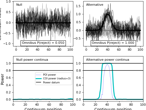
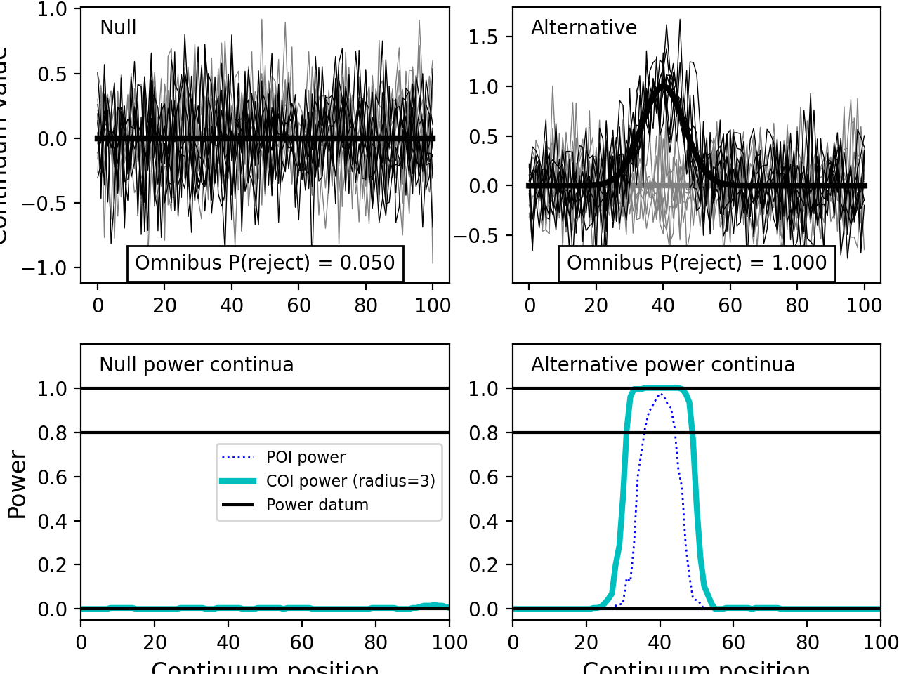
results.plot()
(Source code, png, hires.png, pdf)

Below attributes and methods can be distinguished as follows:
attribute names are followed by “= None”
method names are followed by “( )” with arguments inside the parentheses, and all methods also have code snippets attached.
SimulationResults
- class power1d.results.SimulationResults(model0, model1, Z0, Z1, dt, two_tailed=False, alpha=0.05)
A class containing power1d simulation results including distributions and derived probabilities.
- Q
continuum size
- Z0
test statistic continua (“null” experiment)
- Z1
test statistic continua (“alternative” experiment)
- alpha
Type I error rate (default 0.05)
- coi
continuum centers-of-interest (if any) for which summary powers will be displayed when printing results
- coir
center-of-interest radius (for coi continuum, default 3)
- dt
total simulation duration (s)
- k
cluster extent (default 1); clusters in the excursion set with smaller extents will be ignored when computing probabilities
- model0
the “null” experiment model (an instance of power1d.models.Experiment)
- model1
the “alternative” experiment model (an instance of power1d.models.Experiment)
- niters
number of simulation iterations
- p1d_coi0
COI probability continuum for the “null” experiment
- p1d_coi1
COI probability continuum for the “alternative” experiment
- p1d_poi0
POI probability continuum for the “null” experiment
- p1d_poi1
POI probability continuum for the “alternative” experiment
- p_reject0
omnibus null rejection probability for the “null” experiment (alpha by defintion)
- p_reject1
omnibus null rejection probability for the “alternative” experiment (power by defintion)
- plot(q=None)
Plot simulation results.
This will plot the “null” and “effect” experiment models along with their omnibus powers and their power continua.
By defintion the “null” experiment model will have an omnibus power of alpha and its power continua will be considerably smaller than alpha, with power decreasing as a function of continuum size.
The “effect” experiment model will have an omnibus power that depends on the signal and noise models contained in its DataSample models.
Keyword arguments:
q —— an optional array specifying continuum points (default None)
Example:
>>>  Q = results.Q  #continuum size
>>>  results.plot( q=np.linspace(0, 1, Q) )
- poi
continuum points-of-interest (if any) for which summary powers will be displayed when printing results
- roi
region(s) of interest (default: whole continuum)
- save(filename)
Save simulation results.
Arguments:
filename —— full path to a file. Should have a “.npz” extension (numpy compressed format). It must follow the rules of np.savez.
Example:
>>> results.save( "/Users/username/Desktop/my_results.npz" )
- set_alpha(alpha)
Set the Type I error rate.
After calling this method all probabilities will be re-computed automatically.
Arguments:
alpha —— Type I error rate (float between 0 and 1)
Example:
>>> results.set_alpha( 0.01 )
- set_cluster_size_threshold(k)
Set a cluster size threshold (k) for null hypothesis (H0) rejection.
By default k*=1 is used, in which case only the distribution of the continuum maximum is used as the H0 rejection criterion. For *k larger than one, the H0 rejection criterion becomes defined by the distribution of excursion set (supra-threshold cluster) geometry. In particular, all excursion set clusters with extents less than k are ignored both in critical threshold computations and in power computations.
After calling this method all probabilities will be re-computed automatically.
Arguments:
k —— Type I error rate (integer greater than 0)
Example:
>>> results.set_cluster_size_threshold( w )
- set_coi(*coi)
Set centers-of-interest (COIs) to be displayed when printing.
An arbibtrary number of (location, radius) pairs specifying locations of empirical interest. These COI results will be displayed when using the “print” command as indicated in the example below.
After calling this method all relevant probabilities will be re-computed automatically.
Arguments:
coi —— A sequence of integer pairs (location, radius)
Example:
>>>  results.set_coi( (10,2), (50,8), (85,4) )
>>>  print(results)
- set_coi_radius(r)
Set centers-of-interest (COI) radius for the COI continuum results.
When using the “plot” method COI continuum results will be displayed by default. These indicate power associated with small regions surrounding the particular continuum point.
If the continuum radius is small the COI power will generally be smaller than the omnibus power. As the COI radius increases the COI power will plateau at the omnibus power.
If the continuum radius is one then the COI power continuum is equivalent to the point-of-interest (POI) power continuum.
After calling this method all relevant probabilities will be re-computed automatically.
Arguments:
r —— COI radius (int)
Example:
>>>  results.set_coi_radius( 5 )
>>>  results.plot()
- set_poi(*poi)
Set points-of-interest (POIs) to be displayed when printing.
The power associated with an arbibtrary number of continuum POIs will be displayed when using the “print” command as indicated in the example below.
After calling this method all relevant probabilities will be re-computed automatically.
Arguments:
poi —— A sequence of integers
Example:
>>>  results.set_coi( (10,2), (50,8), (85,4) )
>>>  print(results)
- set_roi(roi)
Set region of interest (ROI).
An ROI constrains the continuum extent of the null hypothesis (H0). By default the entire continuum is considered to be the ROI of interest. Single or multiple ROIs can be specified as indicated below, and this will cause all data outside the ROIs to be ignored.
Setting the ROI to a single point will yield results associated with typical power calculations. That is, a single continuum point behaves the same as a single scalar dependent variable.
After calling this method all probabilities will be re-computed automatically.
Arguments:
roi —— a boolean array or a power1d.continua.RegionOfInterest object
Example:
>>>  Q = results.Q  #continuum size
>>>  roi = np.array( [False]*Q )  #boolean array
>>>  roi[50:80] = True
>>>  results.set_roi( roi )
>>>  print(results)
>>>  results.plot()
- sf(u)
Survival function.
The probability that the “effect” distribution exceeds an arbitrary threshold u.
Arguments:
u —— threshold (float)
Example:
>>>  print(  results.sf( 3.0 )  )
>>>
>>>  u = [0, 1, 2, 3, 4, 5]
>>>  p = [results.sf(uu) for uu in u]
>>>  print( p )
- z0
distribution upon which omnibus H0 rejection decision is based (“null” model)
- z1
distribution upon which omnibus H0 rejection decision is based (“alternative” model)
- zstar
critical threshold for omnibus null (based on Z0max)